Material Balance: example 1, part 2

Oil material balance calculation for a model without a gas cap and aquifer. Fit and Drive indeces.

After estimate STOIP using both, Havlena–Odeh and Campbell diagnostic plots in the first part, link, the cumulative production, \(N_p\) can be simulate to validate the results. With \(w_p =0\) and \(m=0\), the equation is

\[ N_p = \frac{NB_{oi}}{(B_o+(R_p-R_s)B_g)}\left[\frac{(B_o-B_{oi})+(R_{si}-R_s)B_g}{B_{oi}} +\frac{c_wS_{wc}+c_f}{1-S_{wc}} \Delta p \right]\]

Getting \(N=250\) from Campbell plot, add a calculated Np column

N = 250

BM_data <- BM_data %>% 
  mutate(Np_cal  = ((N*Boi)/(Bo+Bg*(Rp-Rs)))*(((Bo-Boi)+(Rsi-Rs)*Bg)/Boi+(Pi-Pavg)*(cw*Sw+cf)/(1-Sw)))

plot_MB_3 <- ggplot(BM_data) + 
  geom_point(aes(x = Date, y = Np)) + 
  geom_line(aes(x = Date, y = Np_cal))

plot_MB_3

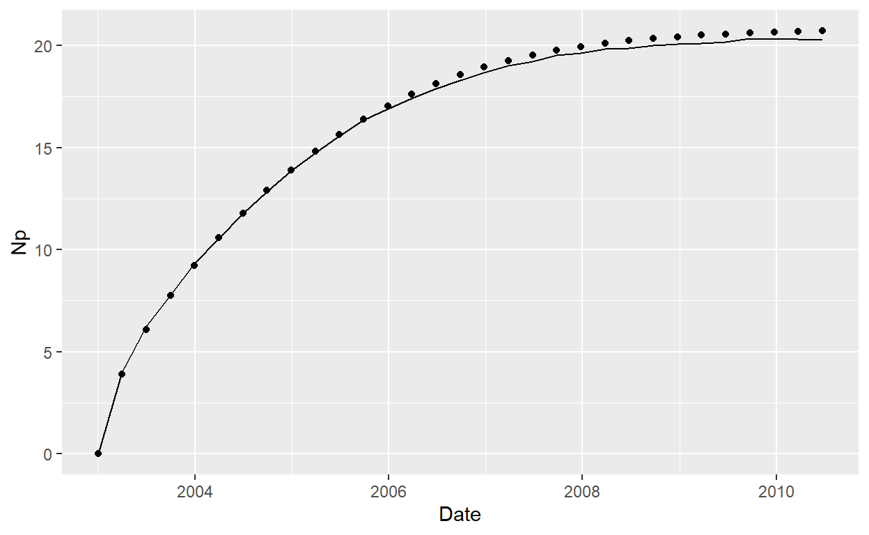
We can observe some different at the end of plot, it can be improve using non-linear regression a estimate a value of \(N\) that fit better \(Np\). With minpack.lm we can use Levenberg-Marquardt algorithm o minimiza the differente. First, we need to define a residual function, in this case, the different between real Np and calcualted. Once getting a fit \(N\) value, we recalculate \(Np\)

library(minpack.lm)

residFun <- function(parS, observed, data, Swf = Sw, cff = cf, cwf = cw, Pif = Pi){
  
  Boif <- data$Bo[1]
  Rsif <- data$Rs[1]
  Pif <- data$Pavg[1]
  
  Np_cal <- ((parS$Nf*Boi)/(data$Bo+data$Bg*(data$Rp-data$Rs)))*
    (((data$Bo-Boif)+(Rsif-data$Rs)*data$Bg)/Boif+(Pif-data$Pavg)*(cwf*Swf+cff)/(1-Swf)) 
  
  #sum(abs(observed - Np_cal))
  observed - Np_cal
}


parStart <- list(Nf = N)

fit_model <- nls.lm(par = parStart, fn = residFun, observed =  BM_data$Np,
                    data = BM_data, Swf = Sw, cff = cf, cwf = cw, 
                    Pif = Pi, control = nls.lm.control(nprint=1))

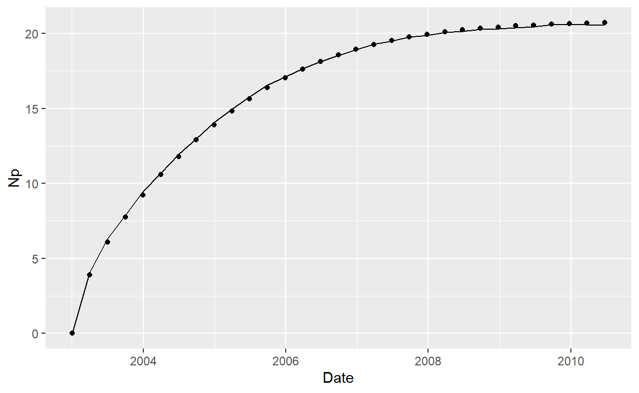
It.    0, RSS =    1.88377, Par. =        250
It.    1, RSS =   0.403168, Par. =    253.265
It.    2, RSS =   0.403168, Par. =    253.265

fit_coeff <- as.list(coef(fit_model))

print(paste("Fit N = ", fit_coeff, sep = ""))

[1] "Fit N = 253.264567990061"

BM_data <- BM_data %>% 
  mutate(Np_cal  = ((fit_coeff$Nf*Boi)/(Bo+Bg*(Rp-Rs)))*
           (((Bo-Boi)+(Rsi-Rs)*Bg)/Boi+(Pi-Pavg)*(cw*Sw+cf)/(1-Sw)))


plot_MB_3 <- ggplot(BM_data) + 
  geom_point(aes(x = Date, y = Np)) + 
  geom_line(aes(x = Date, y = Np_cal))

plot_MB_3

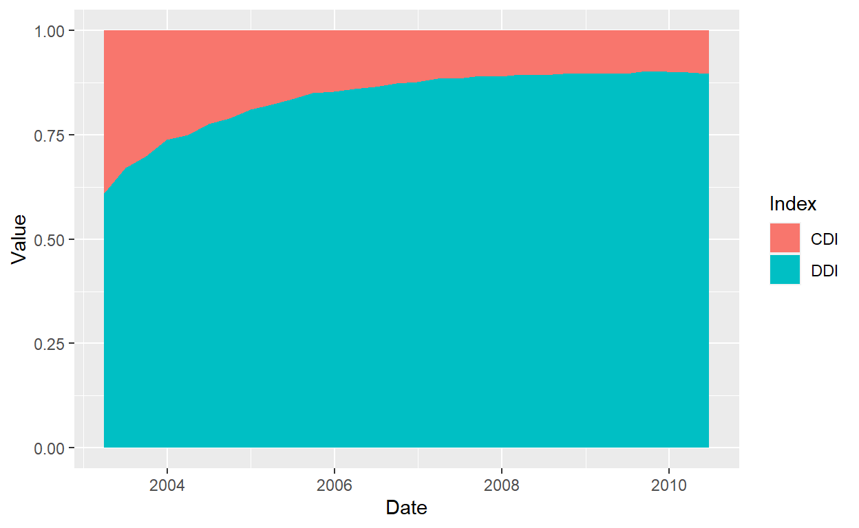
Finally, The drive indices can be calculated using the following equations

Depletion Drive Index \[ DDI = \frac{N[(B_o-B_{oi})+(R_{si}-R_s)B_g]}{N_p(B_o+(R_{si}-R_s)B_g)}\]

Compaction Drive Index

\[CDI = \frac{NB_{oi}(1+m) \left( \frac{c_wS_{wc}+c_f}{1-S_{wc}} \right) \Delta p}{N_p(B_o+(R_{si}-R_s)B_g)}\]

BM_data <- BM_data %>% 
mutate(DDI = ((fit_coeff$Nf*((Bo-Boi)+(Rsi-Rs)*Bg))/(Np*(Bo+Bg*(Rp-Rs)))),
       CDI = 1-DDI)

DDI <- BM_data[,c("Date", "DDI")] 
DDI$Index <- "DDI"

CDI <- BM_data[,c("Date", "CDI")] 
CDI$Index <- "CDI"

colnames(DDI) <- c("Date", "Value", "Index")
colnames(CDI) <- c("Date", "Value", "Index")
Index <- rbind(DDI, CDI)

ggplot(Index, aes(x=Date, y=Value, fill=Index)) +
  geom_area() 

References Sanni, M. (2019) Petroleum Engineering. Principles, Calculatios, and Workflows