A reservoir with initial pressure of 5200 psi and temperature of 123 °F has the following properties:
Porosity = 0.2
\(S_{wc}\) = 0.15
\(c_f\) = 3.50 E-06 \(psi^{-1}\)
\(c_w\) = 7.00 E-06 \(psi^{-1}\)
API = 30°
GOR = 800 scf/stb
\(g_g\) = 0.8
First, loading de production and fluid properties data
Using the following equations we can create Campbell and Havlena-Odeh diagnostic plots
\[F = NE_t+We \quad (1) \]
where
\[ F = N_p(B_o+(R_p-R_s)B_g)+W_pB_w\]
And
\[E_t = B_{oi}\left[\frac{(B_o-B_{oi})+(R_{si}-R_s)}{B_{oi}}+m \left(\frac{B_g}{B_{gi}}-1 \right) + (1+m)\left(\frac{c_wS_{wc}+c_f}{1-S_{wc}}\Delta p\right) \right] \]
Rearranging equation (1)
\[ \frac{F}{E_t} = N + \frac{W_e}{E_t}\]
In Campbell plot case the reservor is volumetric, so \(W_e = 0\) and the indepent term is the oil produced (\(N_p\)) and the first term is the original oil in place (\(N\))
In the Havlena-Odeh diagnostic methos the equation (1) is rearrangin in the following form
\[ F - W_e = NE_t\] Hence, a plot of (\(F-W_e\)) against \(E_t\) will yield a straight-line passing through the origin with slope of the plot giving initial oil in place (\(N\)).
The R code is the following, First we can get the initial \(B_o\) and \(R_s\) and then, using dplyr functions, calculate \(F\) and \(E_t\)
Sw <- 0.15
cf <- 0.0000035
cw <- 0.000007

Boi <- BM_data$Bo[1]
Rsi <- BM_data$Rs[1]
Pi <- BM_data$Pavg[1]

BM_data <- BM_data %>%
  mutate(F = Np*(Bo+Bg*(Rp-Rs)),
         Et = Boi*(((Bo-Boi)+(Rsi-Rs)*Bg)/Boi+(Pi-Pavg)*(cw*Sw+cf)/(1-Sw)),
         F_ET = F/Et)

head(BM_data)
        Date    Pavg    Np   Gp    Bo    Rs    Bg    Rp         F
1 2003-01-01 5200.00  0.00 0.00 1.376 0.800 0.545 0.800  0.000000
2 2003-04-02 3940.89  3.89 3.11 1.389 0.800 0.613 0.800  5.403210
3 2003-07-02 3512.38  6.07 4.85 1.364 0.747 0.651 0.800  8.488913
4 2003-10-01 3322.18  7.74 6.17 1.336 0.696 0.673 0.798 10.871960
5 2003-12-31 3178.82  9.22 7.51 1.316 0.658 0.692 0.814 13.128837
6 2004-03-31 3058.58 10.57 8.98 1.299 0.627 0.709 0.850 15.401621
          Et     F_ET
1 0.00000000      NaN
2 0.02227416 242.5775
3 0.03493341 243.0027
4 0.04382336 248.0860
5 0.05315130 247.0088
6 0.06142994 250.7185
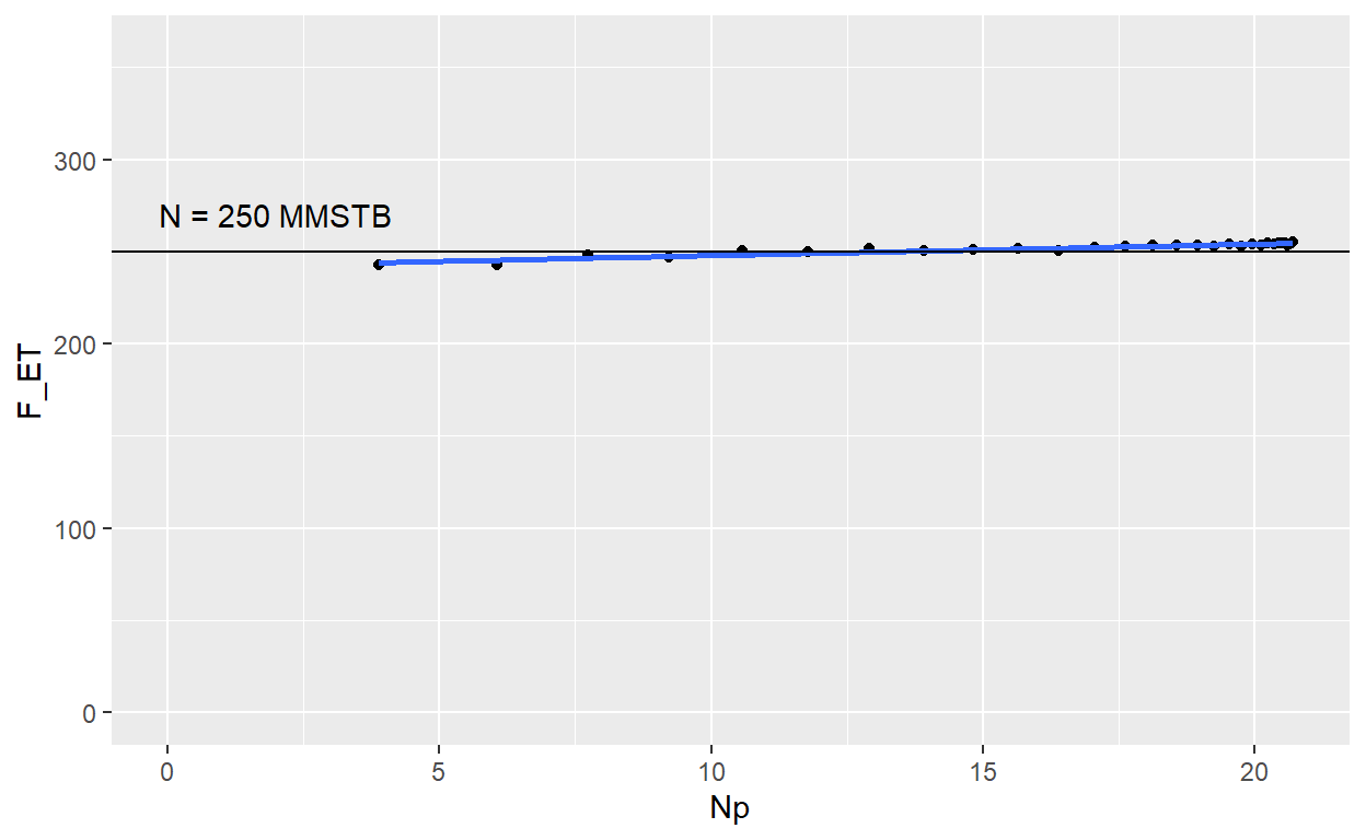
Now, the plots can be generated using ggplot2 package. The Campbell plot shows an horizontal stright-line with an intersection in 250, indicating an approximate 250 MMSTB OOIP
#Campbell plot
plot_MB_1 <- ggplot(BM_data, aes(x = Np, y = F_ET)) +
  geom_point() +
  ylim(0, 360) +
  stat_smooth(method = lm, se = TRUE) +
  geom_hline(yintercept=250) +
  geom_text(aes(x = 2, y = 270, label = "N = 250 MMSTB"),  stat = "unique")

plot_MB_1

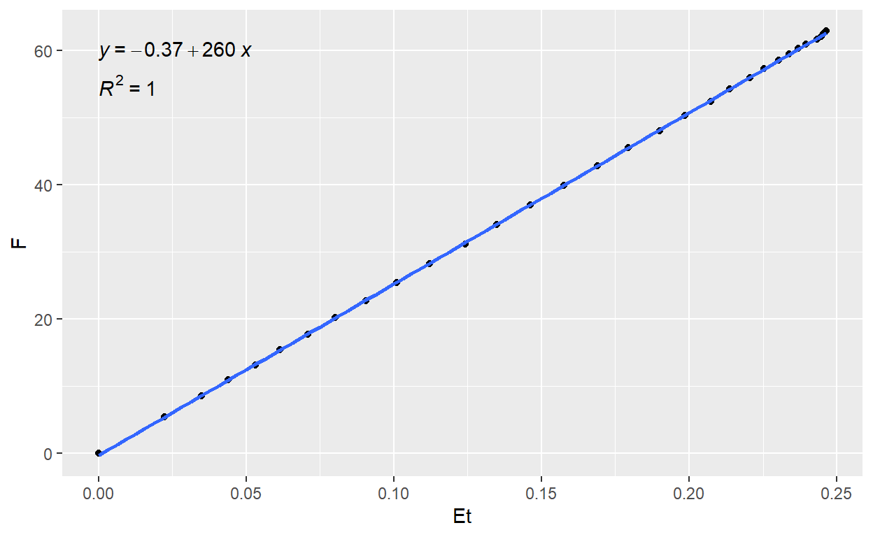
The Havlena–Odeh shows a stright-line with a slope of 260, indicating an approximate 260 MMSTB OOIP. The function stat_regline_equation(), from ggpubr package, let us show the equation from the smoothing
#Havlena–Odeh
plot_MB_2 <- ggplot(BM_data, aes(x = Et, y = F)) +
  geom_point() +
  stat_smooth(method = "lm", se = FALSE) +
  stat_regline_equation(label.y = 60, aes(label = ..eq.label..)) +
  stat_regline_equation(label.y = 55, aes(label = ..rr.label..)) #+
  #geom_hline(yintercept=250) +
  #geom_text(aes(x = 2, y = 270, label = "N = 250 MMSTB"),  stat = "unique")

plot_MB_2

References Sanni, M. (2019) Petroleum Engineering. Principles, Calculatios, and Workflows