Simple linear regression: Y - Function example

Bubble point pressure maybe is the most important result from Constant composition Expansion test. The CCE validation consist in verify measured Bubble point pressure fit with teorical tendency of relative volume and pressure.

The relative volume data frequently require smoothing to correct for laboratory inaccuracies in measuring the total hydrocarbon volume just below the saturation pressure and also at lower pressures. A dimensionless compressibility function, commonly called the Y-function, is used to smooth the values of the relative volume. The function in its mathematical form is only defined below the saturation pressure and is given by the following expression:

\[ Y = \frac{P_{sat}-P}{P(V_{rel})-1}\]

where

\(P_{sat} = saturation \ pressure,\ psi\)

\(P = pressure,\ psi\)

\(V_{rel} = relative \ volumen \ at \ pressure \ p\)

In this example CCE data is fitted using simple linear regression in R to validate the experiment results. First, the CCE data is loaded from CSV file. Dataset has two columns, pressure and relative volume.

CCEdata <- read.csv("CCE.csv")
head(CCEdata)

  pressure     RV
1     1936 1.0000
2     1930 1.0014
3     1928 1.0018
4     1923 1.0030
5     1918 1.0042
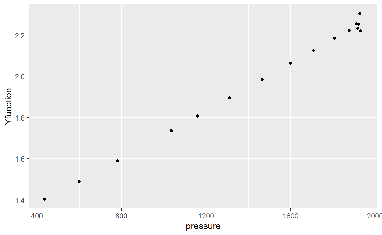
6     1911 1.0058

Using the equation above, Y-fuction is calculated from data and plot it using ggplot2 package

CCEdata$Yfunction <- (max(CCEdata$pressure)-CCEdata$pressure)/(CCEdata$pressure*(CCEdata$RV-1))
head(CCEdata)

  pressure     RV Yfunction
1     1936 1.0000       NaN
2     1930 1.0014  2.220577
3     1928 1.0018  2.305210
4     1923 1.0030  2.253423
5     1918 1.0042  2.234470
6     1911 1.0058  2.255544

library(ggplot2)
ggplot(data = CCEdata, aes(x = pressure, y = Yfunction)) + 
  geom_point()

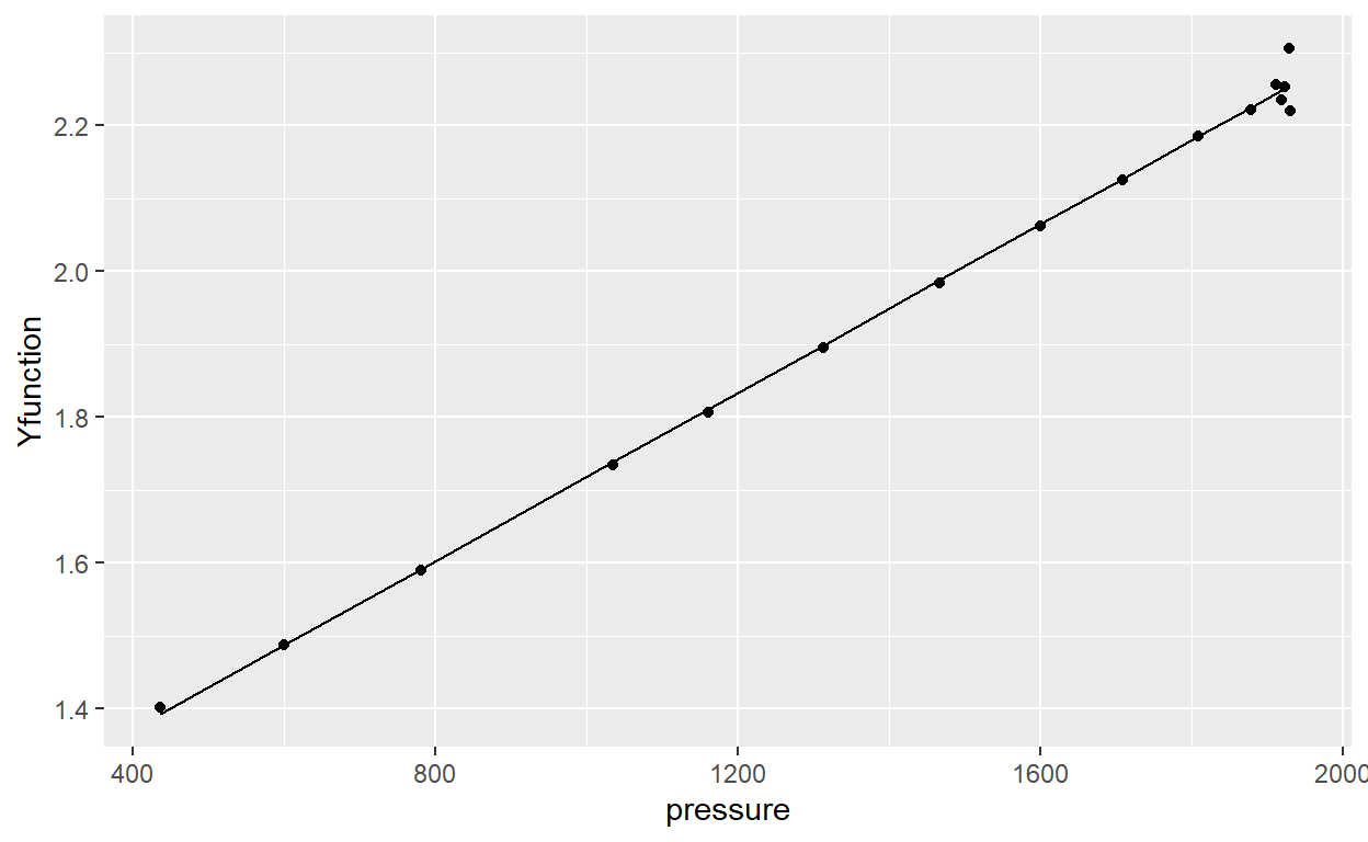
Now, using lm() function, a linear regression model is defined, where the outcome value (y) is the Y-function and the predictor is the pressure (x). Using summary() function, the main characters from model are displayed. We can see that coefficient of determination is very close to 1, which means an excellent fit. Also, Y-function does not show a upper o low trend.

FY_model <- lm(Yfunction ~ pressure, data = CCEdata)
summary(FY_model)

Call:
lm(formula = Yfunction ~ pressure, data = CCEdata)

Residuals:
      Min        1Q    Median        3Q       Max 
-0.034747 -0.004077 -0.002536  0.001464  0.051041 

Coefficients:
             Estimate Std. Error t value Pr(>|t|)    
(Intercept) 1.141e+00  1.359e-02   83.93   <2e-16 ***
pressure    5.776e-04  8.795e-06   65.67   <2e-16 ***
---
Signif. codes:  0 '***' 0.001 '**' 0.01 '*' 0.05 '.' 0.1 ' ' 1

Residual standard error: 0.01755 on 14 degrees of freedom
  (1 observation deleted due to missingness)
Multiple R-squared:  0.9968,    Adjusted R-squared:  0.9965 
F-statistic:  4312 on 1 and 14 DF,  p-value: < 2.2e-16

We can add a column with fitted Y-function values to plot together

CCEdata$Yfunction_fit <- c(NA, FY_model$fitted.values)

head(CCEdata)

  pressure     RV Yfunction Yfunction_fit
1     1936 1.0000       NaN            NA
2     1930 1.0014  2.220577      2.255324
3     1928 1.0018  2.305210      2.254169
4     1923 1.0030  2.253423      2.251281
5     1918 1.0042  2.234470      2.248393
6     1911 1.0058  2.255544      2.244350

ggplot(data = CCEdata) + 
  geom_point(aes(x = pressure, y = Yfunction)) + 
  geom_line(aes(x = pressure, y = Yfunction_fit))

Reference Ahmed, T (2019) Reservoir Engineering Handbook. Fifth edition.