This method combine the Vogel method for oil flow and the constant productivity index for water flow. The IPR curves is determined geometrically from a equations group that consider water and oil flow.
The next figure is used to determine the equation that allow calculate the flowing bottom hole pressure with a total rate.
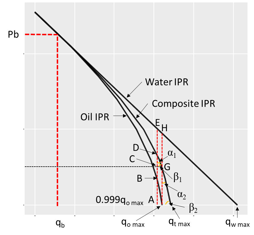
The composite IPR can be divide in 3 regions.
- Between 0 and the flow rate at the bubble point, \(0 < q_t <q_b\) . In this region the rate and flowing bottom hole pressure have a linear relationship.
\[P_{wt}=P_r-\frac{q_t}{J}\]
The region between the flow rate at the bubble point to the maximum oil flow rate, \(q_b < q_t < q_{o max}\) . At a total flow rate, the flowing bottom hole pressure is defined by:
\[P_{wt}=F_o(P_{wtoil})+F_w(P_{wfwater})\]
Using Vogel equation for oil and constant productivity index for water, the flowing bottom hole pressure at the total flow rate is:
\[P_{wt}=F_w(P_r-\frac{q_t}{J})+F_o(0.125)P_b\left[-1+\sqrt{81-80\left[\frac{q_t-q_b}{q_{omax}-q_b}\right]}\right]\]
The interval between the maximum oil flow rate and the maximum total flow rate, \(q_{o max} < q_t < q_{t max}\) . In this interval, the composite IPR curve would have a constant slope, since the curve is mostly affected by water production. So, \(tan \beta\) must be determined for calculating the flowing bottom-hole pressure at a total rate as follows:
- Take a total flow rate is very close to the maximum oil flow rate:
\[q_t=0.999 q_omax\]
Since the difference between \(q_t\) and \(q_{omax}\) is very small, we can assume that \(\alpha_2 = \alpha_1\) and \(\beta_2 = \beta_1\) and the tangent of these angles can be calculated geometrically in the shaded triangle.
From the shaded triangle,
\[tan \beta_1=CD/CG\]
\[tan \alpha_1=CG/CD\]
CD is the difference between the flowing bottom hole pressure at point D, \(P_{wfD}\) and the flowing bottom hole pressure ar point C, \(P_{wfC}\)
\[CD=P_{wfD}-P_{wfc}\]
Point D lies on the composite IPR curve, so:
\[P_{wfD}=F_o(P_{wfoil})+F_w(P_{wfwater})\]
Or, from Figure 1:
\[P_{wfD}=F_o*P_{wfB}+F_w*P_{wfE}\]
\[P_{wfB}=0.125(P_b)*\left[-1+\sqrt{81-80\left[\frac{0.999q_{omax}-q_b}{q_{omax}-q_b}\right]}\right]\]
\[P_{wfE}=P_r-\frac{0.999q_{omax}}{J}\]
Therefore: \[P_{wfD}=F_w\left(P_r-\frac{0.999q_{omax}}{J}\right)+F_o(0.125)P_b*\left[-1+\sqrt{81-80\left[\frac{0.999q_{omax}-q_b}{q_{omax}-q_b}\right]}\right]\]
From Figure 1, \(P_{wfC}=P_{wfG}\) where G also lies on the composite IPR curve for \(qt=q_{omax}\)
\[P_{wfG}=F_o(P_{wfoil}+F_w(P_{wfwater}))\]
At \(q_t=q_{omax}\), \(P_{wfoil}=0\); therefore:
\[P_{wfG}=F_w(P_{wfwater})=F_w\left(Pr-\frac{q_{omax}}{J}\right)\] \[P_{wfC}=P_{wfG}=F_w\left(P_r-\frac{q_{omax}}{J}\right)\]
Substituting equation, yields:
\[CD=P_{wfD}-P_{wfC}=F_w\left(\frac{0.001q_{omax}}{J}\right)+F_o(0.125)P_b\left[-1+\sqrt{81-80\left[\frac{0.999q_{omax}-q_b}{q_{omax}-q_b}\right]}\right]\]
CG is the difference between \(q_t\) and \(q_{omax}\), therefore:
\[CG=q_{omax}-0.999q_{omax}=0.001q_{omax}\]
The maximum total flow rate (for the composite IPR curve) can be calculated by usgin the following equation:
\[q_{tmax}=q_{omax}+F_w(P_r-\frac{q_{omax}}{J})(tan \alpha)\]
Calculation os the total flow rate ar certain flowing bottom-hole pressures for the composite IPR curve
The composite IPR curve can be divided into three intervals, and in every interval, the total flow rate at certain flowing bottom-hole pressures can be calculated as follows:
- For pressures between reservoir pressure and the bubble-point pressure, \(P_b < P_{wf} < P_r\), the toal flow rate can be calculated by using the following equation:
\[q_t=J(P_r-P_{wf})\]
- For pressures between the bubble-point pressure and te flowing bottom-hole pressure where the oil flow rate is equal to the maximum rate, \(P_{efG} < P_{wf} < P_b\), the total flow rate is:
for \(B \neq 0\) \[q_t=\frac{-C+\sqrt{C^2-4B^2}D}{2B^2}\] for \(B=0\) \[q_t=D/C\]
where:
\[A=\frac{P_{wf}+0.125F_oP_r}{0.125F_0P_b}\] \[B=\frac{F_w}{0.125F_oP_bJ}\] \[C=2(A)(B)+\frac{80}{q_{omax}-q_b}\] \[D=A^2-(80)\frac{q_b}{q_{omax}-q_b}-81\]
- For pressures between P{wfg} and 0, that is \(0 < P_{wf} < P_{efG}\), the total flow rate is:
\[q_t=\frac{P_{wfG}+q_{omax}(tan \beta)-P_{wf}}{tan\beta}\]
Example Problem
Reservoir pressure greater than the bubble-point pressure
Give data:
Reservoir pressure, \(P_r=2500 \ psi\) Bubble-point pressure, \(P_b=2100 \ psi\) Test data: Flowing bottom hole pressure = \(P_b=2300 \ psi\) Flow rate (total), \(q_t= 500 \ b/d\)
Calculate: Determine the composite IPR curves for \(F_w = 0.5\)
Code
First, using all the equation above, calculate total flow rates and flowing bottom hole pressure at this rate
library(ggplot2)

Py <- 2550
Pb <- 2100
Pwf <- 2300
Qo <- 500
Fw <- 0.5

#Since Pwf_test > Pb
IP <- Qo/(Py-Pwf)
qb <- IP*(Py-Pb)
qomax <- qb+(2*Pb)/1.8


CD <- (1-Fw)*0.125*Pb*(sqrt(81-80*(0.999*qomax-qb)/(qomax-qb))-1)+
      Fw*(Py-(0.999*qomax)/IP)-Fw*(Py-qomax/IP)

CG <- 0.001*qomax

tana <- CG/CD
tanb <- 1/tana

qtmax <- qomax+Fw*(Py-qomax/IP)*tana
PwfG <- Fw*(Py-qomax/IP)
[1] "j = 2"[1] "qb = 900"[1] "qomax = 3233.33333333333"[1] "tana = 0.409688827872138"[1] "tanb = 2.44087690941891"[1] "qtmax = 3424.521453007"[1] "PwfG = 466.666666666667"Now, we can define some function to do the intervals calculations, with this we can use a \(P_{wf}\) vector to estimate flow rate.
A_IPR_c <- function(Pwf,Fw,Pb,Py){
  A <- (Pwf+0.125*(1-Fw)*Pb-Fw*Py)/(0.125*(1-Fw)*Pb)
  return(A)
}

B_IPR_c <- function(Fw,Pb,J){
  B <- Fw/(0.125*(1-Fw)*Pb*J)
  return(B)
}

C_IPR_c <- function(Pwf,Fw,Pb,Py,J,qomax,qb){
  A <- (Pwf+0.125*(1-Fw)*Pb-Fw*Py)/(0.125*(1-Fw)*Pb)
  B <- Fw/(0.125*(1-Fw)*Pb*J)
  C <- 2*A*B+(80)/(qomax-qb)
  return(C)
}


D_IPR_c <- function(Pwf,Fw,Pb,Pr,J,qomax,qb){
  A <- (Pwf+0.125*(1-Fw)*Pb-Fw*Py)/(0.125*(1-Fw)*Pb)
  D <- A^2-80*(qb/(qomax-qb))-80
  return(D)
}
After that, we can define a \(P_{wf}\) vecto and apply the equation according the intervals
pwf <- c(0,200 ,350 ,600, 1000 ,1400, 1500, 1700, 2100, 2300, 2400, 2550)

A <- A_IPR_c(pwf,Fw,Pb,Py)
B <- B_IPR_c(Fw,Pb,IP)
C <- C_IPR_c(pwf,Fw,Pb,Py,IP,qomax,qb)
D <- D_IPR_c(pwf,Fw,Pb,Py,IP,qomax,qb)

qt <- ifelse(pwf >= Pb, IP*(Py-pwf),
             ifelse(pwf >= PwfG & pwf < Pb,
                    ifelse(rep(B, length(pwf)) != 0 ,
                           (-C+sqrt(C^2-4*B^2*D))/(2*B^2), -D/C),
                    ifelse(pwf < PwfG, (PwfG+qomax*tanb-pwf)/tanb  , 0)))


IPR <- data.frame(pwf = pwf, qt = qt)

ggplot(IPR, aes(x = qt, y = pwf)) +
  geom_line()
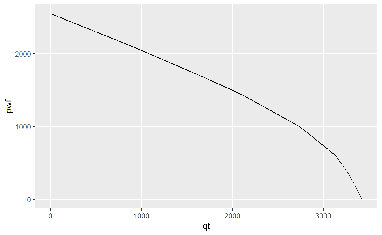
knitr::kable(IPR, caption = "Composite IPR, FW = 0.5")
| pwf | qt |
|---|---|
| 0 | 3424.521 |
| 200 | 3342.584 |
| 350 | 3281.130 |
| 600 | 3135.673 |
| 1000 | 2738.169 |
| 1400 | 2159.923 |
| 1500 | 1995.359 |
| 1700 | 1646.911 |
| 2100 | 900.000 |
| 2300 | 500.000 |
| 2400 | 300.000 |
| 2550 | 0.000 |
Reference: Brown, K. (1984) The technology of artificial lift methods Vol. 4