According to Chan (1995), a log-log plot of WOR (Water - Oil ratio) and its derivatives versus time show different trends for different mechanisms. Chan identified three most noticeable water production mechanisms namely water coning, near well-bore problems and multi-layer channelling.
Water cones upward to the perforations from an underlying water leg or gas cusps downward to the oil zone perforations. Introduction of the second phase into the well stream can occur any time after production has been initiated. Generally, water or gas producing rates increase smoothly as a function of time because of the growth of the cone.
Water or gas channels from a high-permeability layer included in the producing zone. Breakthrough of water or gas is a function of the absolute permeability of the rock layers and the mobility ratio.
Near-wellbore channeling often occurs because of behind pipe communication caused by a bad cement job. WOR or GOR abruptly increases for this case.
Now, we calculate WOR and its derivative using R code, first we have to load the well production data, in this case from a CSV file
  Days   Qo  Qw
1    1  285 385
2    2 1870   7
3    3 3124   1
4    4 2608   1
5    5 3052   5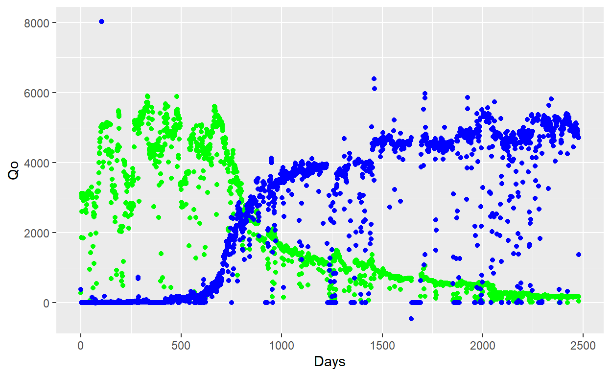
6 6 2983 2ggplot(Prod_data) +
geom_point(aes(x = Days, y = Qo), col = "green") +
geom_point(aes(x = Days, y = Qw), col = "blue")
Now we can add WOR and WOR’ columns, the derivative is calculated with the slope equation.
\[m = \frac{y_2-y_1}{x_2-x_1}=\frac{WOR_2-WOR_1}{t_2-t_1}\] Using diff() function we get the differences between vector elements
Prod_data$WOR <-  Prod_data$Qw/Prod_data$Qo

Prod_data$WORd  <-  c(0, diff(Prod_data$WOR)/diff(Prod_data$Days))

WOR_Data_plot <- data.frame(Days = c(Prod_data$Days, Prod_data$Days),
                            Type = c(rep("WOR", nrow(Prod_data)), rep("WOR'", nrow(Prod_data))),
                            Data = c(Prod_data$WOR, Prod_data$WORd)
                            )

ggplot(WOR_Data_plot, aes(x = Days, y = Data, col = Type)) +
  geom_point(alpha = 0.3) +
  scale_x_log10() +
  scale_y_log10() +
  xlab("Time") +
  ylab("WOR, WOR'") +
  geom_smooth()
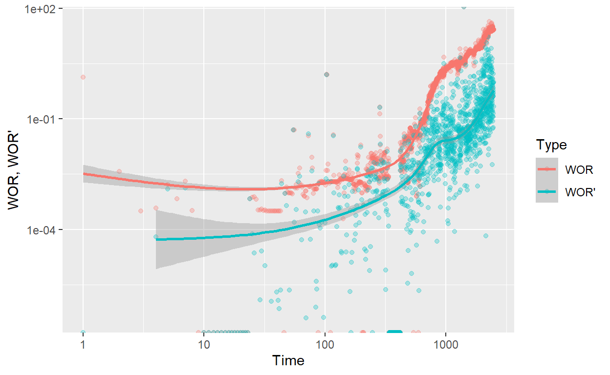
The plot show and gradual increment of WOR and its derivative, using smooth options from ggplot2 package, we can add a trend line. We can consider a probably water coning for water production origin
Reference: Poston, S., Laprea-Bigott, Marcelo and Poe, Bobby (2019) Analysis of oil and gas production perforance