In 1942 Buckley and Leverett developed a model to describe the displacement of one fluid to another in a immiscible way.
The model assummes no mass tranfer between phases, incomplessible fluids and a homogeneous system, the solution gives a saturation profile along the flow direction but ignores capillary pressure and grafity effects.
The fractional flow of a fluid phase, \(f\), is defined as the volumetric flux fraction of the phase that is flowing at position x and time t, fractional flow to water is
\[ f_w = \frac{q_o}{q_o + q_w}\]
Applying Darcy law, for one-dimensional linear flow for simultaneous flow of oil and water, Buckley and Leverett got the following equation
\[ f_w = \frac{1+\frac{Ak\ k_{ro}}{q_t \mu_o}(\frac{\partial P_c}{\partial x}-\Delta \rho g sin \theta)}{1+ \frac{k_{ro} \mu_w}{k_{rw}\mu{o}}}\]
when the flow is in a horizontal reservoir, \(\theta = 0\), the gravity term is absent. Then the fractional flow equation of water phase is reduced to the following
\[ f_w = \frac{1}{1+ \frac{k_{ro} \mu_w}{k_{rw}\mu{o}}}\]
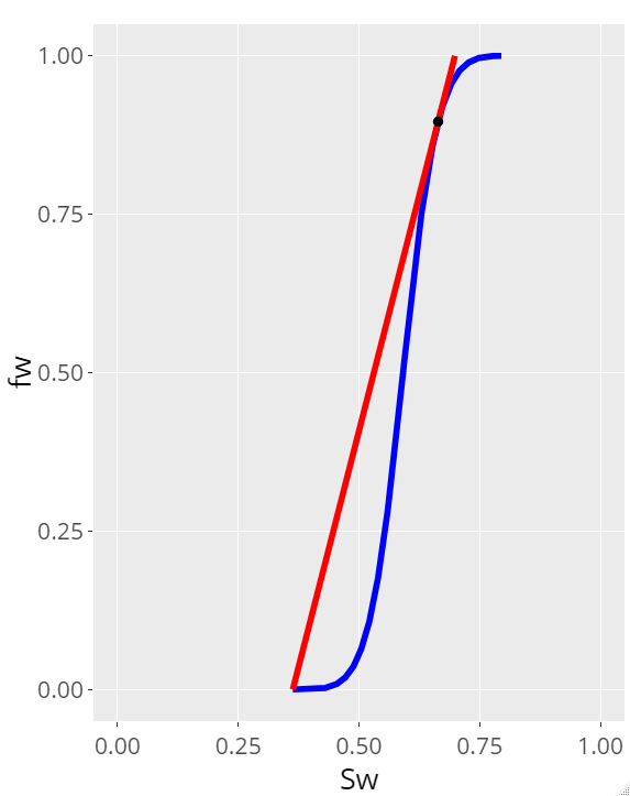
Welge shown a easy approach to estimate the position of the shock saturation front. Draw a line that starts at the point defined by the beginning of water injection to the point of tangency defines the breakthrough or flood front saturation, \(S_{sf}\) and extending the tangency to a 1 \(f_w\) value defines the mean water saturation.
According Welge method we can define \(f_w\) using normalized water saturation \(S_{wD}\) and oil water relative permeability, in this \(k_{ro}\) and \(k_{rw}\) are defined using corey equations. \[ k_{ro} = (1-S_{wD})^n\]
\[ k_{rw} = S_{wD}^m\]
\[ S_{wD} = \frac{S_w - S_{iw}}{1-S_{or}-S_{iw}}\]
\[ f_w = \frac{S_{wD}^{n}}{S_{wD}^{n}+A(1-S_{wD})^m} \]
\[ \frac{\partial f_w}{\partial S_w} = \frac{AB+nS_{wD}^{n-1}(1-S_{wD})^m+mS_{wD}^{n}(1-S_{wD})^{m-1}} {[S_{wD}^{n}+A(1-S_{wD})^m]^2} \]
where
\[ A = \frac{\alpha_1 \mu_w}{\alpha_2 \mu_0}\]
\[ B = \frac{1}{1-S_{or}-S_{iw}}\]
After water breakthrough we can define a production profile with the following calcualtes
- Define a water saturation range after water saturation breakthrough
- Estimate fractional flow mean water saturation in every point
- Compute oil rate
\[ qo = \frac{(1-f_w)q_t}{B_o} \]
- Calculate water-oil ratio
\[ WOR = \frac{f_wB_o}{f_oB_w}\]
- Calculate oil production comulative
\[ N_p = V_p(\overline S_w - S{wi})\]
- Define time
\[ t = \frac{Q_iA\phi L}{q_t}\]
The next example shows the before methodology using R code
\(Reservoir cross Area = 6000 \ ft^2\)
\(Reservoir long = 1000 \ ft\)
\(Porosity = 0.15\)
\(Initial water saturation = 0.363\)
\(Water injection rate = 338 \ B/D\)
\(Oil viscosity = 2 \ cp\)
\(Water viscosity = 2 \ cp\)
\(Oil and water FVF = 1\)
\(relative permeability exponent, no = 2.56, nw = 3.72\)
\(max relative permeability, kromax = 1, krwmax = 0.78\)
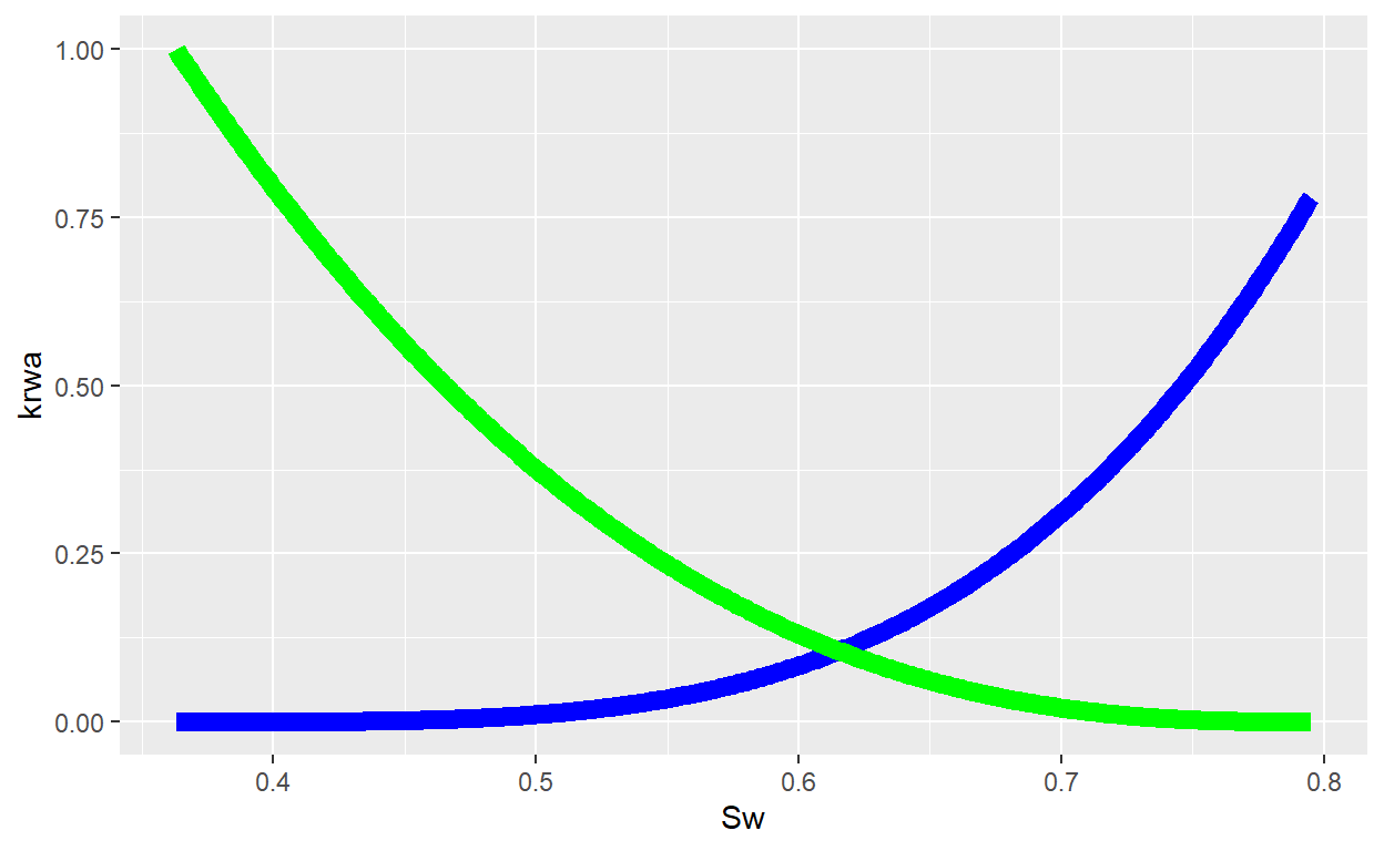
First, define variables from data and generate relative permeability curves to visualize ther behavior
L = 1000
Ar = 6000
Poro = 0.15
K = 100

VisO = 2
VisW = 1
Bo = 1.2
Bw = 1

Sor = 0.205
Swc = 0.363
kromax = 1
krwmax = 0.78
no = 2.56
nw = 3.72

Winj = 338
Swi = 0.363
winjT = 1000

library(ggplot2)
Sw = seq(Swc, (1-Sor), 0.001)
SwD= (Sw - Swc) / (1 - Sor - Swc)
krwa = krwmax * SwD ^ nw
kroa = kromax * (1 - SwD) ^ no

ggplot() +
  geom_line(aes(x = Sw, y = krwa), color = "blue", size = 3) +
  geom_line(aes(x = Sw, y = kroa), color = "green", size = 3)
Now, using Sw vector, estimate de fractional flow in every water saturation point and its slope to get the maximum slope, corresponding to water saturation at breakthrough
A = (kromax * VisW) / (krwmax * VisO)
B = 1/(1 - Sor - Swc)
FWFa = (SwD ^ nw) / ((SwD ^ nw) + (A * (1 - SwD) ^ no))

SwDi = (Swi - Swc) / (1 - Sor - Swc)
FWi = (SwDi ^ nw) / ((SwDi ^ nw) + (A * (1 - SwDi) ^ no))

SLO = ifelse(FWFa > FWi, (FWFa - FWi) / (Sw - Swi),0)

Swbt <- Sw[which.max(SLO)]
Fwbt <- FWFa[which.max(SLO)]
Swbtm = Swbt + ((1 / SLO[which.max(SLO)]) * (1 - FWFa[which.max(SLO)]))

library(plotly)
Fw_fig <- ggplot() +
  geom_line(aes(x = Sw, y = FWFa), color = "blue", size = 1.5) +
  geom_line(aes(x = c(Swi, Swbtm), y = c(FWi, 1)), color = "red", size = 1.5) +
  geom_point(aes(x = Swbt, y = Fwbt), size = 2) +
  geom_point(aes(x = Swbtm, y = 1), size = 2) +
  xlab("Sw") + ylab("fw") +
  theme(text=element_text(size=20)) +
  xlim(0, 1)

ggplotly(Fw_fig)
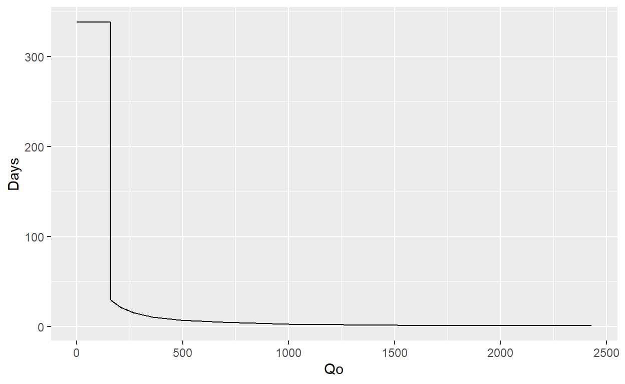
Now, we can define a Sw vector from \(S_{wbt}\) to a any water saturation value, and estimate oil rates and oil production cumulative
SwP <- seq(Swbt, 0.75, length.out = 9)

SwDP= (SwP - Swc) / (1 - Sor - Swc)
krwaP = krwmax * SwDP ^ nw
kroaP = kromax * (1 - SwDP) ^ no

FWFp = (SwDP ^ nw) / ((SwDP ^ nw) + (A * (1 - SwDP) ^ no))

B1=nw*(SwDP^(nw-1))*(1-SwDP)^no
B2=no*SwDP^nw*(1-SwDP)^(no-1)
B3=SwDP^nw+A*(1-SwDP)^no

dFW=(A*B*(B1+B2))/B3^2

td2=1/dFW

SwM=SwP+(td2*(1-FWFp))
Qi=1/dFW

Vp=L*Ar*Poro/5.615;
qw=(FWFp*Winj)/Bw
qo=((1-FWFp)*Winj)/Bo
WOR=FWFp/(1-FWFp)
NP=Vp*(SwM-Swi)
t=(Qi*Vp)/Winj

forecast_data = data.frame(Time = t, Sw = SwP,Fw = FWFp, Swm = SwM, Qi = Qi,
                           Qo = qo, WOR = WOR, Np = NP)

forecast_data
       Time      Sw        Fw       Swm        Qi         Qo
1  159.7426 0.66400 0.8961590 0.6989795 0.3368563 29.2485429
2  204.4821 0.67475 0.9244913 0.7073094 0.4312005 21.2682912
3  267.6916 0.68550 0.9463864 0.7157645 0.5644932 15.1011528
4  358.2731 0.69625 0.9629367 0.7242516 0.7555064 10.4395008
5  490.7674 0.70700 0.9751690 0.7326977 1.0349030  6.9940722
6  690.0936 0.71775 0.9839920 0.7410453 1.4552310  4.5089182
7 1001.6904 0.72850 0.9901773 0.7492486 2.1123090  2.7667334
8 1515.4917 0.73925 0.9943611 0.7572707 3.1957847  1.5882921
9 2430.6904 0.75000 0.9970576 0.7650817 5.1257048  0.8287652
         WOR       Np
1   8.630109 53852.46
2  12.243502 55187.62
3  17.651998 56542.84
4  25.980856 57903.19
5  39.272199 59256.98
6  61.468790 60594.98
7 100.804774 61909.84
8 176.339332 63195.67
9 338.863043 64447.64ggplot() +
geom_line(aes(x = c(0,forecast_data$Time[1], forecast_data$Time),
y = c(Winj,Winj, forecast_data$Qo))) +
xlab("Qo") + ylab("Days")
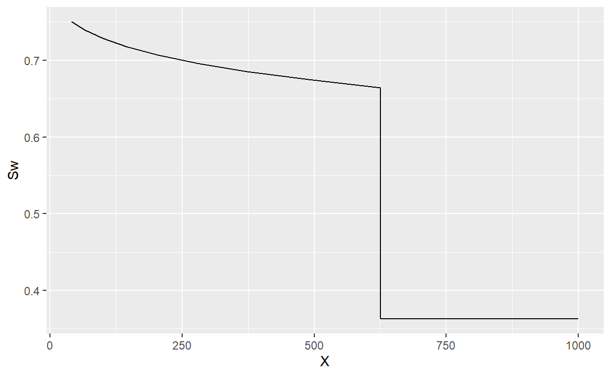
The location \(x_{Sw}\) of any saturation, \(Sw\) can be obtained usaing the following equation
\[ x_{Sw} = \frac{q_tt}{A \phi} \left( \frac{\partial f_w}{\partial S_w} \right)_{Sw} \]
In this case using 100 days
days = 100

XL = dFW*Winj*days*5.6146/(Ar*Poro)

ggplot() +
  geom_line(aes(c(XL, max(XL), L), c(SwP, Swi, Swi))) +
   xlab("X") + ylab("Sw")