Rock typing is the process of splitting the reservoir rock in an specific number of groups according to the petrophysical properties changes, in this example we use core data, porosity and permeability from Volve field. This process is used often in reservoir simulation to group fluid-rock functions, relative permeability and capillary pressure curves.
There are several methods to estimate pore-throat size: Pittman, Winland, Kolodzie and Aguile, most of them fit the pore-throat size from mercury injection capillary pressure experiment at a certain mercury saturation, using linear regression.
In this example, we use Winland correlation to estimate pore-throat size and then, group according this parameter.
\[ log(R35) = 0.588\ log(k) - 0.588\ log(\phi)- 0.966\]
where:
\(R35 = pore \ throat \ radius \ at \ mercury \ saturation \ of \ 35%, \ microns\)
\(k = air-permeability, \ md\)
\(\phi = porosity, \ fraction\)
First, the data is loaded from a CSV file
import pandas as pd

data = pd.read_csv('Core_data.csv')
data
WELL MD POROSITY PERMEABILITY
0 WELL_1 4038.350098 0.201 1973.9240
1 WELL_1 4038.850098 0.203 1158.9270
2 WELL_1 4039.350098 0.207 1935.1169
3 WELL_1 4039.850098 0.206 1003.6810
4 WELL_1 4040.350098 0.190 901.4980
.. ... ... ... ...
401 WELL_2 3918.350098 0.207 31.1830
402 WELL_2 3918.600098 0.198 29.8160
403 WELL_2 3918.850098 0.166 9.8900
404 WELL_2 3919.100098 0.202 31.8940
405 WELL_2 3919.350098 0.150 2.9790
[406 rows x 4 columns]Using above equation, the PTS (pore-throat size) is estimated
import math
import numpy as np

data["PTS"] = 10**(0.588*np.log10(data.PERMEABILITY) - 0.864*np.log10(data.POROSITY) - 0.996)

data
WELL MD POROSITY PERMEABILITY PTS
0 WELL_1 4038.350098 0.201 1973.9240 34.969780
1 WELL_1 4038.850098 0.203 1158.9270 25.350609
2 WELL_1 4039.350098 0.207 1935.1169 33.696552
3 WELL_1 4039.850098 0.206 1003.6810 23.001544
4 WELL_1 4040.350098 0.190 901.4980 23.156673
.. ... ... ... ... ...
401 WELL_2 3918.350098 0.207 31.1830 2.974578
402 WELL_2 3918.600098 0.198 29.8160 3.010631
403 WELL_2 3918.850098 0.166 9.8900 1.832323
404 WELL_2 3919.100098 0.202 31.8940 3.078629
405 WELL_2 3919.350098 0.150 2.9790 0.987667
[406 rows x 5 columns]Once we have the PTS parameter, a categorical variable could be created using the following subdivision, using cut() function from Pandas
| Pore-throat radius, microns | Rock Type |
|---|---|
| <0.1 | Nano |
| 0.1-0.5 | Micro |
| 0.5-2 | Meso |
| 2-10 | Macro |
| >10 | Mega |
data["RT"] = pd.cut(data.PTS, bins = [0,0.1,0.5,2,10,10000000],
                    labels = ["Nano", "Micro", "Meso", "Macro", "Mega"])
data["RT_n"] = pd.cut(data.PTS, bins = [0,0.1,0.5,2,10,10000000],
                      labels = [1,2,3,4,5])

data
WELL MD POROSITY PERMEABILITY PTS RT RT_n
0 WELL_1 4038.350098 0.201 1973.9240 34.969780 Mega 5
1 WELL_1 4038.850098 0.203 1158.9270 25.350609 Mega 5
2 WELL_1 4039.350098 0.207 1935.1169 33.696552 Mega 5
3 WELL_1 4039.850098 0.206 1003.6810 23.001544 Mega 5
4 WELL_1 4040.350098 0.190 901.4980 23.156673 Mega 5
.. ... ... ... ... ... ... ...
401 WELL_2 3918.350098 0.207 31.1830 2.974578 Macro 4
402 WELL_2 3918.600098 0.198 29.8160 3.010631 Macro 4
403 WELL_2 3918.850098 0.166 9.8900 1.832323 Meso 3
404 WELL_2 3919.100098 0.202 31.8940 3.078629 Macro 4
405 WELL_2 3919.350098 0.150 2.9790 0.987667 Meso 3
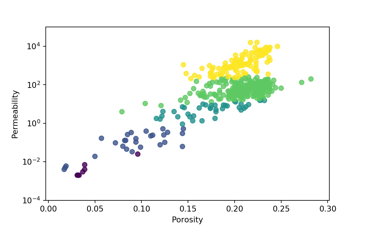
[406 rows x 7 columns]Now, we can plot porosity vs permeability, mapping by rock types, using matplotlib library
import matplotlib.pyplot as plt

plt.scatter(data.POROSITY,data.PERMEABILITY, c = data.RT_n, alpha=0.8);
plt.xlabel('Porosity');
plt.ylabel('Permeability');
plt.yscale('log');
plt.ylim(0.0001,100000);
plt.show();