Survey calculation methods: part 1

The tangential method in R

There are several methods of computing directional surveys, in this case two methods are rewired: Tangential angle and Average angle

The tangential method uses the inclination and azimuth at the lower survey station assuming to be a straight line. The angles measured at the upper station are not used in the computing. This method is the most inaccurate when the trajectory is changing significantly between stations.

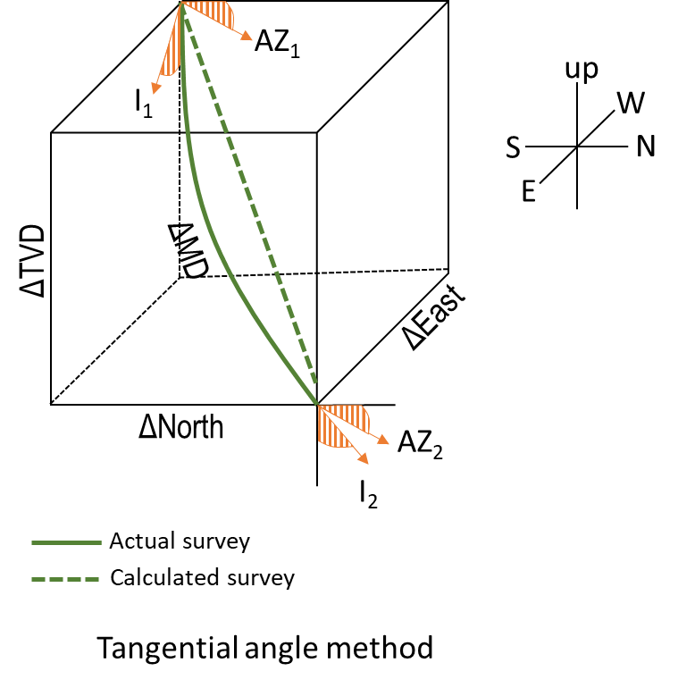
Tangential calcularions:

\[ \Delta North = \Delta MD * sin(I2) * cos(Az2) \]

\[ \Delta East = \Delta MD * sin(I2) * sin(Az2) \]

\[ \Delta TVD = \Delta MD * cos(I2)\]

where

\(MD = measured \ depth \ between \ surveys \ (m)\)

\(I2 = Inclination \ (angle) \ of \ lower \ survey \ (°)\)

\(Az2 = azimuth \ direction \ of \ lower \ survey \ (°)\)

R code

First, loading the survey data from CSV file, in this case we have: MD in meters, Inclination and Azimuth in angles, using read.csv tha data is loaded in dataframe format.

survey <- read.csv("Survey.csv")

head(survey)

  MD        INC        AZ
1  0 0.00000000   0.00000
2 15 0.03000000  86.60000
3 30 0.06000000  86.60000
4 45 0.01550349  96.85197
5 60 0.03000000 256.00000
6 75 0.02455922 247.22631

For this method, two vectors are created, I2 and A2, to Inclination and azimuth of lower survey. With these vectors, just use the equation above to compute $ North$, $ East$ and $ TVD$.

I2 <- survey$INC[2:(nrow(survey))]
A2 <- survey$AZ[2:(nrow(survey))]

survey$TVD <- -c(survey$MD[1], cumsum(diff(survey$MD)*cos(((I2))*pi / 180)))
survey$DN <- c(0, cumsum(diff(survey$MD)*sin(((I2))*pi / 180)*cos(((A2))*pi / 180)))
survey$DE <- c(0, cumsum(diff(survey$MD)*sin((( I2 ))*pi / 180)*sin((( A2 ))*pi / 180)))

head(survey)

  MD        INC        AZ       TVD            DN          DE
1  0 0.00000000   0.00000   0.00000  0.0000000000 0.000000000
2 15 0.03000000  86.60000 -15.00000  0.0004657911 0.007840157
3 30 0.06000000  86.60000 -29.99999  0.0013973733 0.023520469
4 45 0.01550349  96.85197 -44.99999  0.0009131392 0.027550284
5 60 0.03000000 256.00000 -59.99999 -0.0009869108 0.019929599
6 75 0.02455922 247.22631 -74.99999 -0.0034757540 0.014001255

Using Plotly package, the survey can be ploted in 3D

library(plotly)

plot_ly(survey, x = ~DE, y = ~DN, z = ~TVD, type = "scatter3d" , mode = "lines")

We can define a Kelly bushing and head values, as a servey start point, and computing the geographic coordinates and TVDSS

X <- 550000
Y <- 2500000
KB <- 33

survey$TVDSS <- survey$TVD + KB
survey$X <- X + survey$DN
survey$Y <- Y + survey$DE

head(survey)

  MD        INC        AZ       TVD            DN          DE
1  0 0.00000000   0.00000   0.00000  0.0000000000 0.000000000
2 15 0.03000000  86.60000 -15.00000  0.0004657911 0.007840157
3 30 0.06000000  86.60000 -29.99999  0.0013973733 0.023520469
4 45 0.01550349  96.85197 -44.99999  0.0009131392 0.027550284
5 60 0.03000000 256.00000 -59.99999 -0.0009869108 0.019929599
6 75 0.02455922 247.22631 -74.99999 -0.0034757540 0.014001255
      TVDSS      X       Y
1  33.00000 550000 2500000
2  18.00000 550000 2500000
3   3.00001 550000 2500000
4 -11.99999 550000 2500000
5 -26.99999 550000 2500000
6 -41.99999 550000 2500000

plot_ly(survey, x = ~X, y = ~Y, z = ~TVDSS, type = "scatter3d" , mode = "lines")

Reference Inglis, T.A. (1987) Directional Drilling. Petroleum engineering and development studies, Vol. II.