At pressures less than the bubble point pressure, oil flow decreases due to oil relative permeability is reduced because solutions gas escapes and become free gas, increasing oil viscosity also. Because of that IPR curve deviates from linear behavior at pressure less than the bubble-point pressure.
Vogel offered a simplified solution for two-phase flow problem, defined the following equation:
\[q=q_{max}\left[1-0.2\left(\frac{P_{wf}}{P}\right)-0.8\left(\frac{P_{wf}}{P}\right)^{2}\right] \ \ (1)\]
or
\[ p_{wf} = 0.125p\left[\sqrt{81-80\left( \frac{q}{q_{max}} \right) } -1 \right] \ \ (2)\]
where \(q_{max}\) is defined as the absolute open flow (AOF), the maximum possible reservoir deliverability, and its equation is
\[q_{max}=\frac{J^{*}p}{1.8} \ \ (3)\]
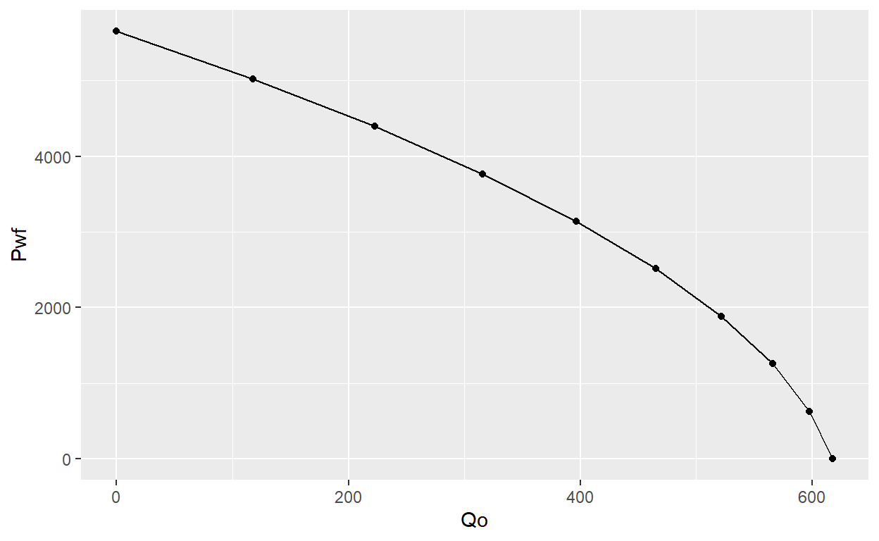
Example. Calculate and graph the IPR for a vertical well in a saturated oil reservoir using Vogel’s equation
\(Porosity = 0.19\)
\(Permeability: k = 8.2 \ md\)
\(Pay \ zone \ thickness: h = 53 \ ft\)
\(Reservoir \ pressure: P_e = 5651 \ psi\)
\(Bubble-point \ pressure: p_b=5651 \ psia\)
\(Oil \ formation \ volume \ factor: B_o=1.1\)
\(Oil \ viscosity: \mu _o = 1.7 \ cp\)
\(Total compressibility: c_t = 0.0000129 \ psi^{-1}\)
\(Drainage \ area: A = 640 \ acres \ (re=2980 \ ft)\)
\(Wellbore \ radius: r_w=0.328 \ ft\)
\(Skin \ factor: S=0\)
First, calculate Productivity index using pseudo-steady state PI equation
py <-  5651
pb <-  5651
k <- 8.2
h <- 53
Bo <- 1.1
viso <- 1.7
re <- 2980
rw <- 0.328
S <- 0

#Productivity index

J = (k*h)/(141.2*Bo*viso*(log(re/rw)-3/4+S))
print(J)
[1] 0.1967785Now, we can estimate AOF and then oil rates using a flowing botton-hole pressure vector to generate the IPR curve
qmax <- (J*py)/1.8
qmax
[1] 617.7751#create a pressure vector from reservoir pressure to zero
pwf <- seq(0,py, length.out = 10)
#Using equation 1 and Productivity index value, calculate Qo
qo <- qmax*(1-0.2*(pwf/py)-0.8*(pwf/py)^2)
#Using Pwf and Qo vector we cna create a dataframe
IPR <- data.frame(Pwf = pwf, Qo = qo)
print(IPR)
         Pwf       Qo
1     0.0000 617.7751
2   627.8889 597.9452
3  1255.7778 565.9125
4  1883.6667 521.6767
5  2511.5556 465.2380
6  3139.4444 396.5963
7  3767.3333 315.7517
8  4395.2222 222.7041
9  5023.1111 117.4535
10 5651.0000   0.0000
Now we can plot IPR with ggplot2
When reservoir pressure is greater than the bubble-point pressure and the flowing bottom-hole pressure can be less than the bubble-point pressure in some conditions, the model have to combine the straight-line IPR for single-phase flow and the Vogel’s IPR model for two-phase flow.
The flow rate at the bubble-point pressure using the linar IPR model is
\[q_b = J(\bar p-p_b)\]
The total flow rate, considering the additional q_b rate and using the Vogel’s IPR model at a given bottom-hole pressure less than the \(P_b\) is expressed as
\[ q = J(\bar p-p_b)+ \frac{J^{*}p}{1.8}\left[1-0.2\left(\frac{P_{wf}}{P}\right)-0.8\left(\frac{P_{wf}}{P}\right)^{2}\right]\]
where
\[\frac{J^{*}p}{1.8}=q_v \ \ (3)\]
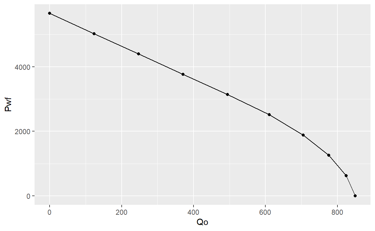
Example. Calculate and graph the IPR for a vertical well in an undersaturated oil reservoir using Vogel’s equation
\(Porosity = 0.19\)
\(Permeability: k = 8.2 \ md\)
\(Pay \ zone \ thickness: h = 53 \ ft\)
\(Reservoir \ pressure: P_e = 5651 \ psi\)
\(Bubble-point \ pressure: p_b=3000 \ psia\)
\(Oil \ formation \ volume \ factor: B_o=1.1\)
\(Oil \ viscosity: \mu _o = 1.7 \ cp\)
\(Total compressibility: c_t = 0.0000129 \ psi^{-1}\)
\(Drainage \ area: A = 640 \ acres \ (re=2980 \ ft)\)
\(Wellbore \ radius: r_w=0.328 \ ft\)
\(Skin \ factor: S=0\)
First, calculate Productivity index using pseudo-steady state PI equation
py <-  5651
pb <-  3000
k <- 8.2
h <- 53
Bo <- 1.1
viso <- 1.7
re <- 2980
rw <- 0.328
S <- 0

#Productivity index

J = (k*h)/(141.2*Bo*viso*(log(re/rw)-3/4+S))
print(J)
[1] 0.1967785Now, we can estimate \(q_b\) and \(q_v\), then oil rates using a flowing botton-hole pressure vector to generate the IPR curve, in this using ifelse() function to evaluate if \(p_{wf}\) is less or grater than \(p_b\)
qb <- (J)*(py-pb)
qb
[1] 521.6597qv <- J*pb/1.8
qv
[1] 327.9641#create a pressure vector from reservoir pressure to zero
pwf <- seq(0,py, length.out = 10)
#Using equation 1 and Productivity index value, calculate Qo
qo <- ifelse(pwf >= pb, J*(py-pwf), qb + qv*(1-0.2*(pwf/pb)-0.8*(pwf/pb)^2))
#Using Pwf and Qo vector we cna create a dataframe
IPR <- data.frame(Pwf = pwf, Qo = qo)
print(IPR)
         Pwf       Qo
1     0.0000 849.6238
2   627.8889 824.4023
3  1255.7778 776.1945
4  1883.6667 705.0004
5  2511.5556 610.8200
6  3139.4444 494.2201
7  3767.3333 370.6650
8  4395.2222 247.1100
9  5023.1111 123.5550
10 5651.0000   0.0000
Now we can plot IPR with ggplot2
References
Guo, Boyun (2008) Well productivity handbook