Inflow performance relationship: Part 1

Generating IPR curve for single and two-phase reservoirs

The IPR curve is a graphical presentation of the relationship between the flowing botton-hole pressure and the liquid production rate. The magnitud of the slope of IPR curve is called productivity index ($PI$ or $J$), expressed as:

$$J=\frac{q}{P_e-P_{wf}} \ \ (1)$$

For undersaturated oil reservoir or reservoir regions where the pressure is greater than the bubble-point pressure we can use the following equations

““For radial transient flow around a vertical well””

$$J^*=\frac{q}{(P_e-P_{wf})}=\frac{kh}{162.6B_o\mu_o(logt+log \frac{k}{\phi\mu_oc_tr^{2}_w}-3.23+0.87S)}$$ ““For radial steady-state flow around a vertical well”” $$J^*=\frac{q}{(P_e-P_{wf})}=\frac{kh}{141.2B_o\mu_o(In\frac{r_e}{r_w}+S)}$$ \For pseudo-steady-state flow around a vertical well\ $$J^*=\frac{kh}{141.2B_o\mu_o(In\frac{r_e}{r_w}-\frac{3}{4}+S)}\\J^*=\frac{q}{(P-P_{wf})}=\frac{kh}{141.2B_o\mu_o(\frac{1}{2}In\frac{4A}{\gamma{C_A}r^{2}_w}+S)}$$ \For steady-state flow around a fractured well\ $$J^*=\frac{q}{(P_e-P_{wf})}=\frac{kh}{141.2B_o\mu_o(In\frac{r_e}{r_w}+S_f)}$$ \For steady-state flow around a horizontal well\ $$j^{*}=\frac{q}{(P_e-P_{wf})}=\frac {k_Hh} {141.2B_o\mu_o\left[In\left[\frac{a+\sqrt{a^{2}-(L/2)^{2}}}{L/2}\right]+\frac{1_{ani}h}{L}In\left[\frac{1_{ani}h}{r_w(1_{ani}+1)}\right]\right]}$$

Example in R

Using the following data we can calculate and graph the IPR for a vertical well in an oil reservoir considering pseudo-steady state flow.

$Porosity = 0.19$

$Permeability: k = 8.2 \ md$

$Pay \ zone \ thickness: h = 53 \ ft$

$Reservoir \ pressure: P_e = 5651 \ psi$

$Bubble-point \ pressure: p_b=5651 \ psia$

$Oil \ formation \ volume \ factor: B_o=1.1$

$Oil \ viscosity: \mu _o = 1.7 \ cp$

$Total compressibility: c_t = 0.0000129 \ psi^{-1}$

$Drainage \ area: A = 640 \ acres \ (re=2980 \ ft)$

$Wellbore \ radius: r_w=0.328 \ ft$

$Skin \ factor: S=0$

py <-  5651
k <- 8.2
h <- 53
Bo <- 1.1
viso <- 1.7
re <- 2980
rw <- 0.328
S <- 0

#Productivity index

J = (k*h)/(141.2*Bo*viso*(log(re/rw)-3/4+S))
print(J)

[1] 0.1967785

IPR points to graph can be calculated as follow

#create a pressure vector from reservoir pressure to zero

pwf <- seq(0,py, length.out = 10)

#Using equation 1 and Productivity index value, calculate Qo

qo <- J*(py-pwf)

#Using Pwf and Qo vector we cna create a dataframe

IPR <- data.frame(Pwf = pwf, Qo = qo)
print(IPR)

         Pwf        Qo
1     0.0000 1111.9951
2   627.8889  988.4401
3  1255.7778  864.8851
4  1883.6667  741.3301
5  2511.5556  617.7751
6  3139.4444  494.2201
7  3767.3333  370.6650
8  4395.2222  247.1100
9  5023.1111  123.5550
10 5651.0000    0.0000

Now we can plot IPR with ggplot2

library(ggplot2)

ggplot(IPR, aes(x = Qo, y = Pwf)) + 
  geom_point() + geom_line()

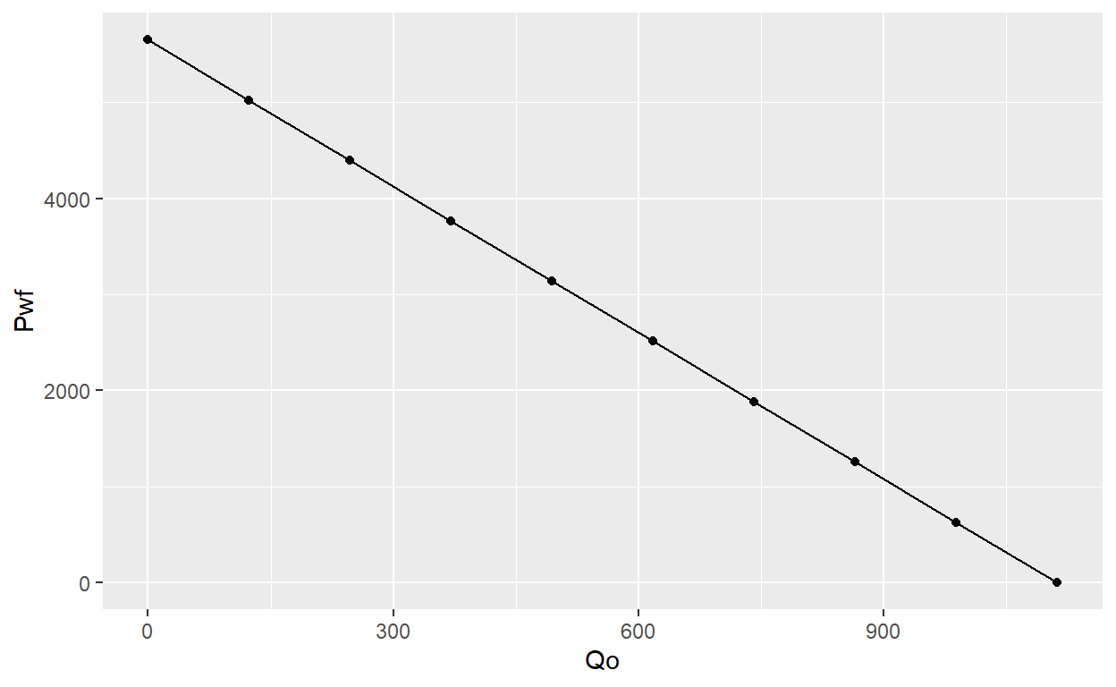
The last IPR model us valid for pressure above bubble-point pressure.

With the last code we can create a function to automate IPR calculations, if you want to know more about functions in R check the this link, Define function in R

Darcy_PSS <- function(py,k,h,Bo,viso,re,rw,S){
  
  J = (k*h)/(141.2*Bo*viso*(log(re/rw)-3/4+S))
 
  pwf <- seq(0,py, length.out = 10)

  qo <- J*(py-pwf)

  IPR <- data.frame(Pwf = pwf, Qo = qo)

return(IPR)

}

IPR <- Darcy_PSS(4500, 8.2,53,1.1,1.7,2980,0.328,0)
print(IPR)

    Pwf        Qo
1     0 885.50310
2   500 787.11387
3  1000 688.72464
4  1500 590.33540
5  2000 491.94617
6  2500 393.55693
7  3000 295.16770
8  3500 196.77847
9  4000  98.38923
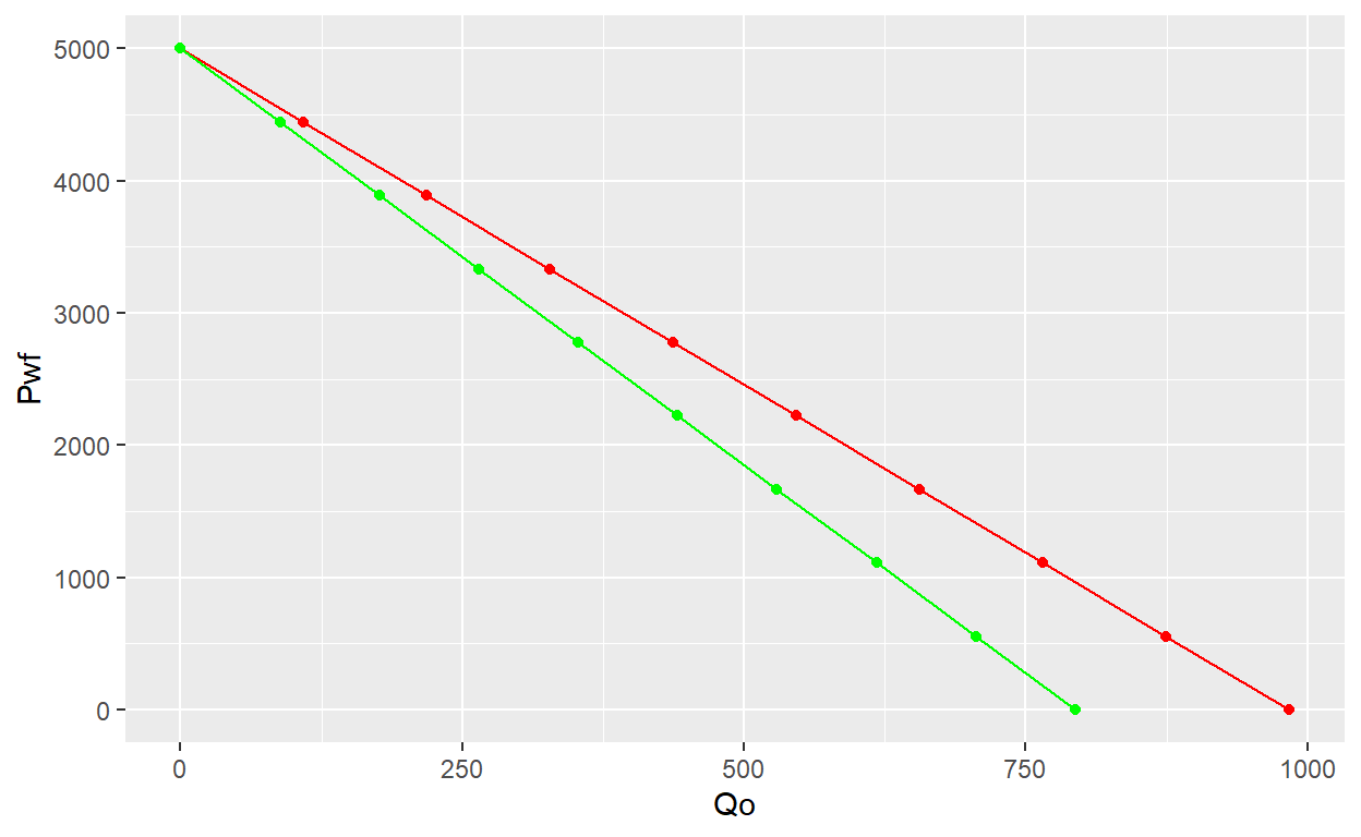
10 4500   0.00000

Now we can compare IPR with and without skin easily

IPR_nS <- Darcy_PSS(5000, 8.2,53,1.1,1.7,2980,0.328,0)
IPR_S <- Darcy_PSS(5000, 8.2,53,1.1,1.7,2980,0.328,2)

ggplot() + 
  geom_point(data = IPR_nS, aes(x = Qo, y = Pwf), color = "red") + 
  geom_line(data = IPR_nS, aes(x = Qo, y = Pwf), color = "red")+ 
  geom_point(data = IPR_S, aes(x = Qo, y = Pwf), color = "green") + 
  geom_line(data = IPR_S, aes(x = Qo, y = Pwf), color = "green")

References

Guo, Boyun (2008) Well productivity handbook

Buy me a coffee