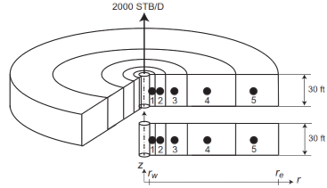
A 0.5-ft-diameter wáter well is located in 20-acre spacing. The reservoir thickness, horizontal permeability, and porosity are 30 ft, 150 md, and 0.23, respectively. The flowing fluid has FVF, compressibility and viscosity of 1 RB/B, 1 x 10^-5, and 0.5 cP, respectively. The external boundaries are no-Flow boundaries. The well has open-well completion and is placed on production at a rate of 2000 B/D. Initial reseroir pressure is 4000 psia. The reservoir can be simulated using five gridblocks in the radial direction.Find the pressure distribution in the reservoir after 1 day and 3 days.
#Reservoir simulation example. 1D radial coordinates, one phase only and homogeneous
library(plotly)
library(reshape2)

#input data

nx <- 5   #number of cells
beta <- 0.001127  #convertion factor
alpha <- 5.614  #convertion factor

re <- 526.6040 #Reservoir external radius, ft
h <- 30 #ft, dimension in z direction

#Rock and fluid data
poro <- 0.23 #porosity, fraction
Cr <- 0 #rock Compressibility psi^-1
Cf <- 0.00001 #fluid Compressibility  psi^-1
k <- 150 #permeability, md
Bo <- 1 #Formation volume factor, RB/STB
vis <- 0.5 #viscosity,cp

#Well information
rw <- 3 #in, well radius
s <- 0 #skin
cellP <- 1 #well cell
qo <- -2000 #well rate, STB/D

dt <- 1 #time step, days
TT <- 3 #total simulation time

Po <- 4000 #psi, Initial condition
Grid node and its data are calculated using the following equation:
Geometrical factor \[ \alpha_{lg} = \left(\frac{re}{rw}\right)^{1/n_r}\] First node radius \[ r_1 = [\alpha_{lg}ln(\alpha_{lg})/(\alpha_{lg}-1)]r_w\] Nodes radius \[ r_{i+1} = \alpha_{lg}r_i\]
Face blocks radius
\[ r_{i+1}^L = \frac{r_{i+1}-r_{i}}{ln(r_{i+1}/r_{i})} \]
#location gridblocks
al2 <-  (re / (rw / 12))^(1 / nx) #alpha, geometrical factor
rn <- 0
rn[1]  <-  (al2 / (al2 - 1)) * log(al2) * (rw / 12)

for (i in 2:nx){
  rn[i] <-  al2 * rn[i - 1]
}

#face blocks radius
rf <- 0
for (i in 1:nx-1){
  rf[i] <-  (rn[i + 1] - rn[i]) / log(rn[i + 1] / rn[i])
}

rf[nx]  <-  re

#Cells volume
vol <- 0
vol[1] <-  3.1416 * (rf[1] ** 2 - (rw / 12) ** 2) * h
for(i in 2:nx){
  vol[i] = 3.1416 * (((rf[i]) ** 2) - ((rf[i-1]) ** 2)) * h
}

#Faces area
Ax = 2 * 3.14 * rf[1] * h
The past data is used to estimate transmissibility and acumulation terms.
Geometrical factor
\[ G_{ri} = \frac {2 \pi \beta kh}{ln(\alpha_{lg})}\]
Transmissibility in the \(r\) direction
\[ T_{ri} = G_{ri} \left( \frac{1}{\mu B} \right) \]
#Geometrical factor
Gr <- (2*pi*beta*k*h)/(log(al2))
TE <-  Gr*(1/(vis * Bo)) #  East transmisibility
TW <-  Gr*(1/(vis * Bo)) #  West transmisibility

Acum <- ((vol * poro * (Cf + Cr)) / (alpha * Bo * dt))
time <- dt
Pt <- rep(Po, nx) #Pressure at time n
Ptdt <- rep(0, nx) #Pressure at time n + 1

#geometry well factor

FG <- (2 * 3.1416 * beta * k * h) / (log(rn[1] / (rw / 12)) + s)

#Results data.frame
results_cells <- data.frame(0, t(Pt))
colnames(results_cells) <- c("Time", 1:nx)
cells_x <- rn #seq(dx/2, (dx*nx)-(dx/2), length.out = nx)

results_pwf <- data.frame(Time = numeric(), Pwf = numeric())
We have to define thomas algorithm function to solve tridiagonal matrix.
thomas <- function(a,b,c,d,x,n){
  # Subroutine to solve a tridiagonal system
  # a = subdiagonal vector
  # B = diagonal vector
  # c = superdiagonal vector
  # d = right hand side vector
  # x = solution vector
  # n = number of diagonal vector elements

  #Forward elimination
  for(i in 2:n){
    b[i] <- b[i]-a[i]*c[i-1]/b[i-1]
    d[i] <- d[i]-a[i]*d[i-1]/b[i-1]
  }

  #Back substitution
  x[n] <- d[n]/b[n]
  for(i in (nx-1):1){
    x[i] <- (d[i]-c[i]*x[i+1])/b[i]
  }

  return(x)
}
Once we have defined the geometry and the equations terms, we can begin the time loop, where we have to define de vector for thomas algoriths and get the pressure in the next time
#Time loop
while( time <= TT ){

  aa <- rep(TW, nx)
  bb <- -(TW + TE + Acum)
  cc <- rep(TE, nx)
  dd <- -Acum*Pt

  #Boundary condition, No flow
  #West
  bb[1] <- -(TE + Acum[1])
  #East
  bb[nx] <- -(TW + Acum[nx])

  #Well
  dd[cellP] = dd[cellP] - qo

  Ptdt <- thomas(aa,bb,cc,dd,Ptdt,nx)

  Pt <- Ptdt

  pwf = qo / (FG / (Bo * vis)) + Pt[cellP]
  results_cells <- rbind(results_cells, c(time,Ptdt))
  results_pwf <-rbind(results_pwf, c(time, pwf))
  time = time + dt
}
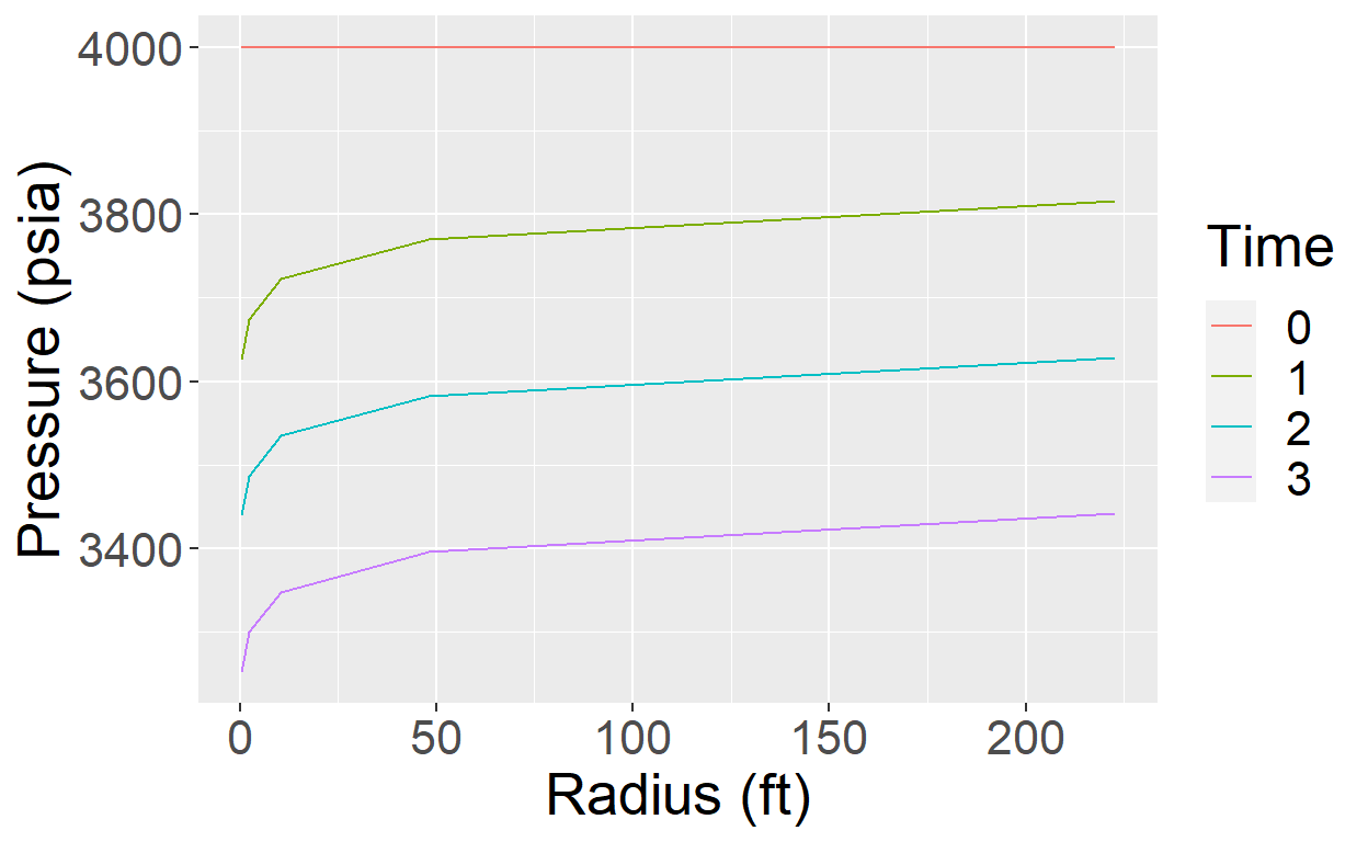
At the end we just generate some plots to visualize the results
#Plot
options(repr.plot.width=16, repr.plot.height=8)
results_cells_time <- reshape2::melt(results_cells,id.vars=c("Time"))
colnames(results_cells_time) <- c("Time", "Radius", "Pressure")
results_cells_time$Time <- as.factor(results_cells_time$Time)
results_cells_time$Radius <- rep(rn, each = nrow(results_cells))

ggplot(results_cells_time, aes(Radius, Pressure, color = Time)) +
       geom_line() +
       xlab("Radius (ft)") + ylab("Pressure (psia)") +
       theme(text = element_text(size=20))
print(results_cells)
  Time        1        2        3        4        5
1    0 4000.000 4000.000 4000.000 4000.000 4000.000
2    1 3626.282 3674.314 3722.337 3770.211 3815.447
3    2 3438.930 3486.961 3534.988 3582.915 3628.691
4 3 3252.142 3300.173 3348.201 3396.127 3441.910print(results_cells_time)
   Time      Radius Pressure
1     0   0.4883173 4000.000
2     1   0.4883173 3626.282
3     2   0.4883173 3438.930
4     3   0.4883173 3252.142
5     0   2.2563731 4000.000
6     1   2.2563731 3674.314
7     2   2.2563731 3486.961
8     3   2.2563731 3300.173
9     0  10.4260485 4000.000
10    1  10.4260485 3722.337
11    2  10.4260485 3534.988
12    3  10.4260485 3348.201
13    0  48.1757596 4000.000
14    1  48.1757596 3770.211
15    2  48.1757596 3582.915
16    3  48.1757596 3396.127
17    0 222.6062736 4000.000
18    1 222.6062736 3815.447
19    2 222.6062736 3628.691
20    3 222.6062736 3441.910
Reference
Abou-Kassem, J., Farouq, S. M. & Rafiq, M. (2006) Reservoir simulation. A basic approach. Gulf Publising Compana.