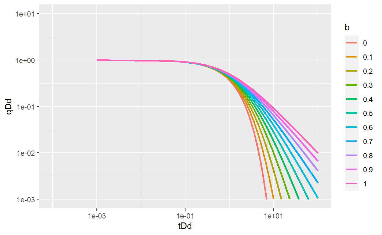
The type curve matching analysis method is one of different methods to determine the decline parameters: \(b\), \(q_i\) and \(D_i\)
Other methods could be trial and error, and curve matching, etc.
Dimensionless time
\[t_{Dd} = D_it\]
Dimensionless rate, exponential declina
\[q_{Dd} = \frac{q}{q_i}=e^{-t_{Dd}}\]
hyperbolic decline
\[q_{Dd} = (1+bt_{Dd})^{-1/b} \ \text{b is constant,} \ 0<b<1\]
harmonic decline
\[q_{Dd}= \frac{1}{1+t_{Dd}}\] Using the equation above, we can generate and plot type curve. Define \(t_{Dd}\) values and \(b\) value from 0 to 1. With lapply() function we can repeat \(q_{Dd}\) calculate with every \(b\) value, the result is a list that we can convert in a single dataframe
With melt() function from reshape2 package we can melt the dataframe in less columns, in this case put all \(q_{Dd}\) in a single column. Finally plot \(q_{Dd}\) Vs. \(t_{Dd}\) and grouping by \(b\) value
library(ggplot2)
library(reshape2)
library(plotly)

tDd <- c(seq(0.001,100,0.05))
b <- seq(0,1,0.1)
qDd_la <- lapply(b, function(b)
  if(b == 0){
    exp(-tDd)
  }else{
    (1+b*tDd)^(-1/b)
  }

  )

qDd <- data.frame(qDd_la)
colnames(qDd) <- b
qDd$tDd <- tDd
qDd <- reshape2::melt(qDd,id.vars="tDd")
colnames(qDd) <- c("tDd","b","qDd")

fet_plot <- ggplot() +
  #geom_line(data = qDd_tr,aes(tDd_t,qDd_tr,group = reD, col = reD),size = 1) +
  geom_line(data = qDd,aes(tDd,qDd,group = b, col = b),size = 1) +
  xlab("tDd") +
  ylab("qDd") +
  scale_y_log10(limits = c(0.001, 10)) +
  scale_x_log10(limits = c(0.0001, 100))

fet_plot

ggplotly(fet_plot)