Schmalz and Rahme (1950) introduced a single parameter that describes the degree of heterogeneity within a pay zone section. The term is called Lorenz coefficient and varies between zero, for a completely homogeneous system, to one for a completely heterogeneous system. The following steps summarize the methodology of calculating Lorenz coefficient:
Step 1. Arrange all the available permeability values in a descending order.
Step 2. Calculate the cumulative permeability capacity \(\sum{kh}\) and cumulative volume capacity \(\sum{{\phi}h}\).
Step 3. Normalize both cumulative capacities such that each cumulative capacity ranges from 0 to 1.
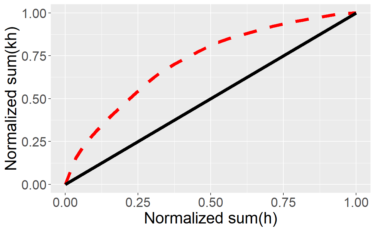
Step 4. Plot the normalized cumulative permeability capacity versus the normalized cumulative volume capacity on a Cartesian scale.
The coefficient is defined by the following expression: \[L = \frac{\text{Area above the straight line}}{\text{Area below the straight line}}\] where the Lorenz coefficient L can vary between 0 and 1. 0 = completely homogeneous 1 = completely heterogeneous
Example 4.20 (Ahmed, 2019)
Tabulate the permeability data in a descending order and calculate the normalized \(\sum{kh}\) and \(\sum{h}\). Using the mutate function from dplyr package, we add the normalized data in the original dataframe
We add zeros at the first row usind rbind function to combine zeros vector with dataframe and get a curve from zero. Then generate a dateframe to plot straight line from (0,0) to (1,1)
v.0 <- c(0,0,0,0,0,0,0)
data.LC <- rbind(v.0, data.LC)

stringi.line <- data.frame(h.n = c(0,1), kh.n = c(0,1))
ggplot(data.LC, aes(h.n, kh.n)) +
  geom_line(size = 2, color = "red", linetype = "dashed") +
  geom_line(data = stringi.line, aes(h.n, kh.n), size = 2) +
  theme(text = element_text(size=20)) +
  xlab("Normalized sum(h)") +
  ylab("Normalized sum(kh)")
To calculate area under de curve we can use AUC (Area Under the Curve) function from DescTools package, calculating the area under the curve from a vector of x-y coordinates. Then we can use the Lorenz coefficient equation above
kh.auc <- AUC(data.LC$h.n, data.LC$kh.n, from = 0, to = 1)

Lorenz.coeff <- (kh.auc-0.5)/0.5
print(paste("L = ", Lorenz.coeff))
[1] "L = 0.435086404514195"Reference Ahmed, T (2019) Reservoir Engineering Handbook. Fifth edition.