Logistic Growth Model(LMG) model

Hubbert used the LGM approach to predict the cumulative production from gas and oil fields or region

Hubbert (1956) was the first to employ the concept of LGM (Logistic Growth Model) in the oil industry. Hubbert used the LGM approach to predict the cumulative production from gas and oil fields or regions. Clark et al. (2011) proposed a three-parameter growth model to forecast the production growth from a production well; that is, cumulative oil “NP” or gas “GP.” Clark and co-authors proposed the following expression:

For cumulative oil \("Np"\) or gas \("Gp"\) \[Gp = \frac{(K)t^n}{a+t^n}\] For oil rate \("Qo"\) or gas rate \("Qg"\) \[Q_g = \frac{(K)nat^{n-1}}{(a+t^n)^2}\] The parameters \("a"\) and \("n"\) are regression variables that impact the shape and upwards and downward of the decline curve. The “K” acts as a bounded or maximum growth.

Data and example 18.7 (Ahmed, 2019)

Matching observed production data using LGM method

Load data from .csv file

library(ggplot2)
library(plotly)
library(dplyr)
library(ggpubr)
library(crosstalk)
library(minpack.lm)
library(DT)

gas_rate <- read.csv("REH_Ch_18.csv")

datatable(gas_rate)

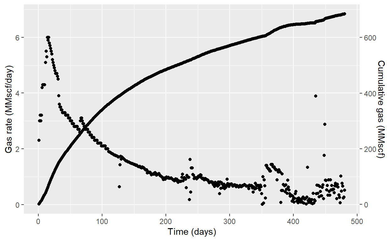
fig <- ggplot() + 
       geom_point(data = gas_rate, aes(DAYS,RATE), color = "black") +
       geom_point(data = gas_rate, aes(DAYS,GP/100), color = "black") +
       ylab("Gas rate (MMscf/day)") + xlab("Time (days)") +
       scale_y_continuous(sec.axis = sec_axis(~ . * 100, name="Cumulative gas (MMscf)"))  
                          


fig

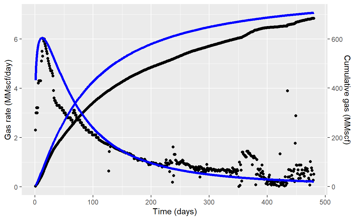
Assuming the following values for the three LMG parameters:

\[K = 800\] \[N = 1.2\] \[a = 220\]

gas_rate <- gas_rate %>%
            mutate(Qg_cal = (800 * 1.2 * 220 * DAYS^(1.2-1))/(220 + DAYS^1.2)^2,
            Gp_cal = (800 * DAYS^(1.2))/(220 + DAYS^1.2))


fig <- fig + geom_line(data = gas_rate, aes(gas_rate$DAYS,gas_rate$Qg_cal), color = "blue", size = 1.5) +
             geom_line(data = gas_rate, aes(gas_rate$DAYS,gas_rate$Gp_cal/100), color = "blue", size = 1.5)

fig

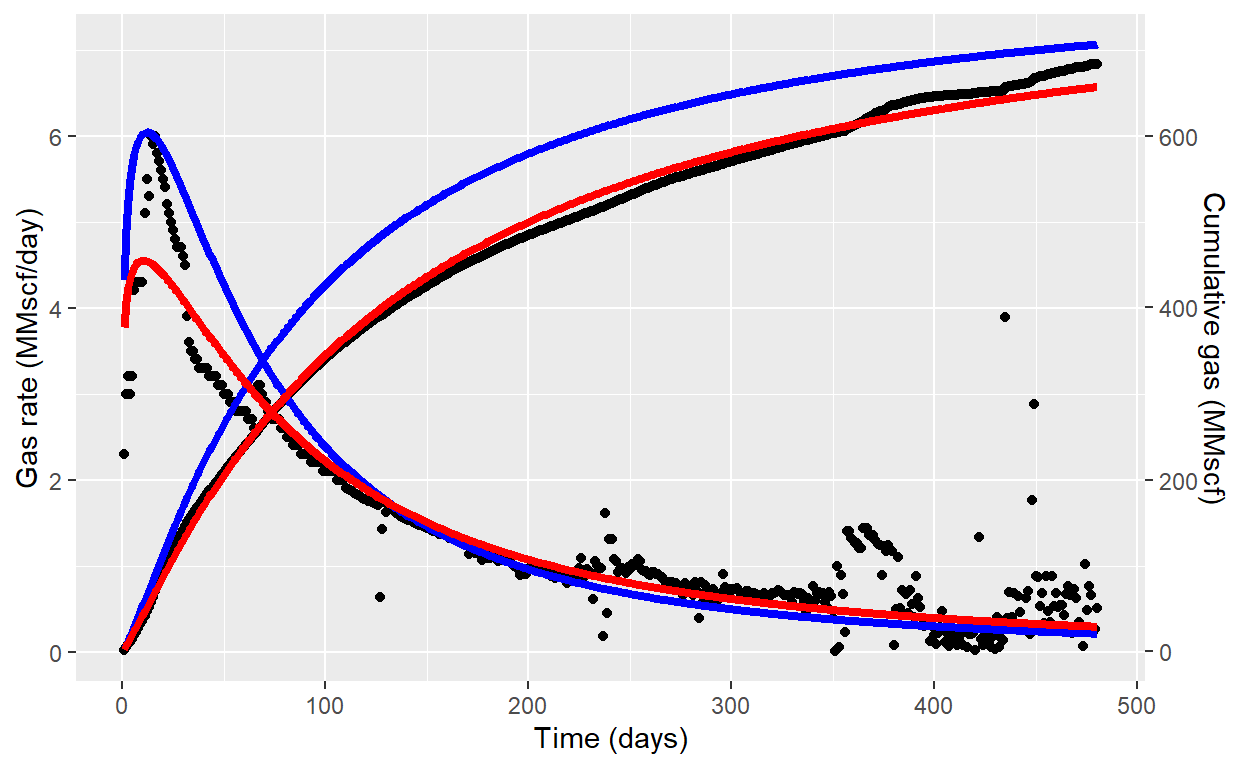
We can use non-linear regression with minpack.lm package using

dca.LGM <- nlsLM(
  RATE ~ (K.cal*n.cal*a.cal*DAYS^(n.cal-1))/(a.cal+DAYS^n.cal)^2,
  data = gas_rate,
  start = list(
    K.cal = 800,
    a.cal = 220,
    n.cal = 1.2
    
  )
)

coefficients(dca.LGM)

     K.cal      a.cal      n.cal 
808.044750 239.005696   1.124712 

gas_rate$Qg_reg <- fitted(dca.LGM) 
gas_rate$Gp_reg <- (coefficients(dca.LGM)[1]*gas_rate$DAYS^(coefficients(dca.LGM)[3]))/
                   (coefficients(dca.LGM)[2]+gas_rate$DAYS^coefficients(dca.LGM)[3])

fig <- fig + geom_line(data = gas_rate, aes(DAYS,Qg_reg), color = "red", size = 1.5) +
             geom_line(data = gas_rate, aes(DAYS,Gp_reg/100), color = "red", size = 1.5)

fig

datatable(gas_rate)

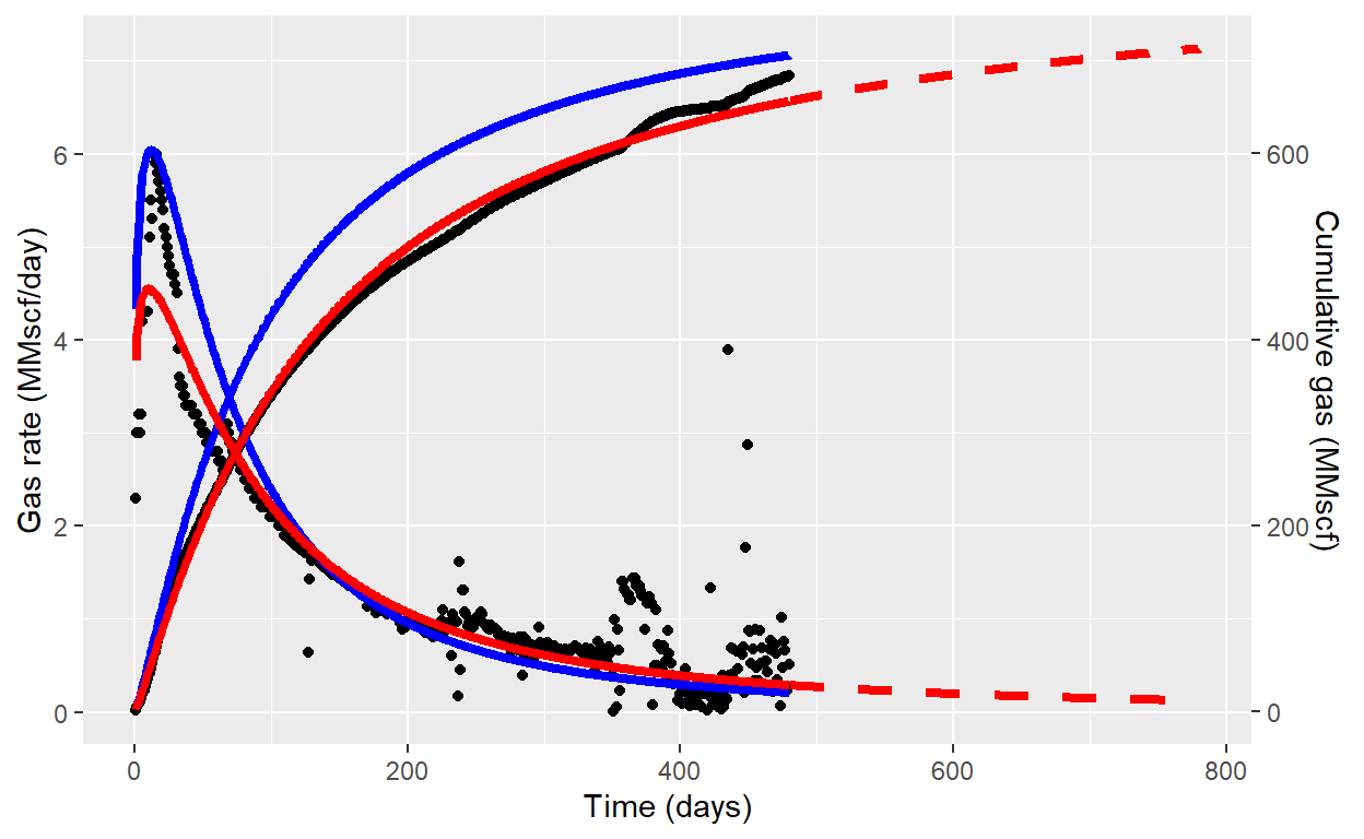
For generate a forecast, we can create a days vector and calculate rates using model equation and fit coefficients. Initially, creating a dataframe with forecasting data and then, using merge() function merge both dataframes, in this case, because both have DAYS column the function just add Qg_for and Gp_for columns and fill empty rows with NA values.

K <- coefficients(dca.LGM)[1]
a <- coefficients(dca.LGM)[2]
n <- coefficients(dca.LGM)[3]


days_forc <- c(481:780)
rate_forc <- (K*n*a*days_forc^(n-1))/(a+days_forc^n)^2
gp_forc <- (K*days_forc^(n))/(a+days_forc^n)

forcast <- data.frame(DAYS = days_forc, Qg_for = rate_forc, Gp_for = gp_forc)

gas_rate_for <- merge(gas_rate, forcast, all = TRUE)

fig <- fig + geom_line(data = forcast, aes(DAYS,Qg_for), color = "red", size = 1.5, linetype = "dashed") +
             geom_line(data = forcast, aes(DAYS,Gp_for/100), color = "red", size = 1.5,linetype = "dashed")

fig

Files

Reference Ahmed, T (2019) Reservoir Engineering Handbook. Fifth edition.