Shale content methods

Exercise 5.1 Sensitivity on Vsh Calculation Ref. Sanni, M. (2019) Petroleum Engineering. Principles, Calculatios, and Workflows

Gamma Ray logs can be used for determining the shale content in a formation using differents relationship between Vsh and GR. Data.

Vsh Calculation Methods (Sanni, 2019).

Method	Formula	Formulation and comments
Linear (Gamma Ray Index)	\[V_{sh} = I_{GR}\]	Based in linear relationship between shale volume and GR response
Larionov [1969] for tertiary (unconsolidated) rock	\[V_{sh} = 0.083(2^{3.7I{GR}}-1)\]	Based on empirical correlation. Linear relationship overestimates \(V_{sh}\) for tertiary (unconsolidated) rocks.
Larionov (1969) for pre-tertiary (older and consolidated) rock	\[V_{sh} = 0.33(2^{2I{GR}}-1)\]	Based on empirical correlation. Linear relationship overestimates \(V_{sh}\) pre-tertiary (consolidate) rocks
Stieber [1970]	\[V_{sh}=\frac{0.5I_{GR}}{1.5-I_{GR}}\]	Calibration to Gulf coast log
Clavier et al. [1971]	\[V_{sh}=1.7-(3.38-(I_{GR}+0.7)^2)^{1/2}\]	Compromise between Larionov Tertiary and old rock model

\(I_{GR}\) is called the gamma ray index and it is defined as: \[I_{GR} = \frac{GR_{Zone}-GR_{Clean}}{GR_{Shale}-GR_{Clean}}\]

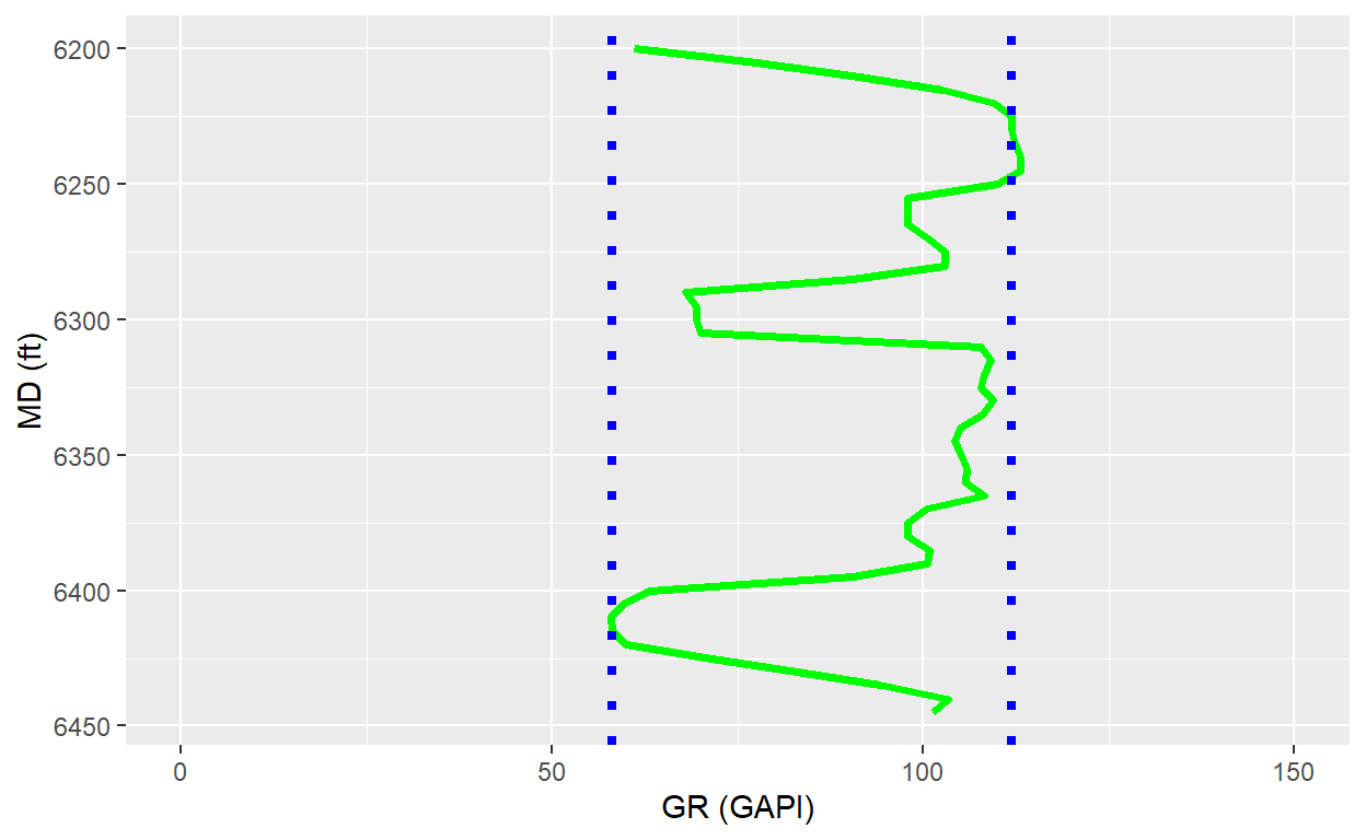
First, read the log data and plot the GR log

library(ggplot2)
library(dplyr)
library(DT)
library(plotly)

log_data <- read.csv("Ex_5.1_log.csv")

datatable(log_data)

fig <- ggplot(log_data) + geom_line(aes(MD,GR), color = "green", size = 1.25) +
                   coord_flip() + ylab("GR (GAPI)") + xlab("MD (ft)") +
                   scale_x_continuous(trans = "reverse") +
                   scale_y_continuous(position = "right") + ylim(0, 150)

fig

According GR plot we can define as \(GR_{Shale} = 111.86\) and \(GR_{Clean} = 58.12\)

fig <- fig + geom_hline(yintercept = 58.12, linetype="dotted", 
                color = "blue", size=1.5) + 
            geom_hline(yintercept = 111.86, linetype="dotted", 
                color = "blue", size=1.5)

fig

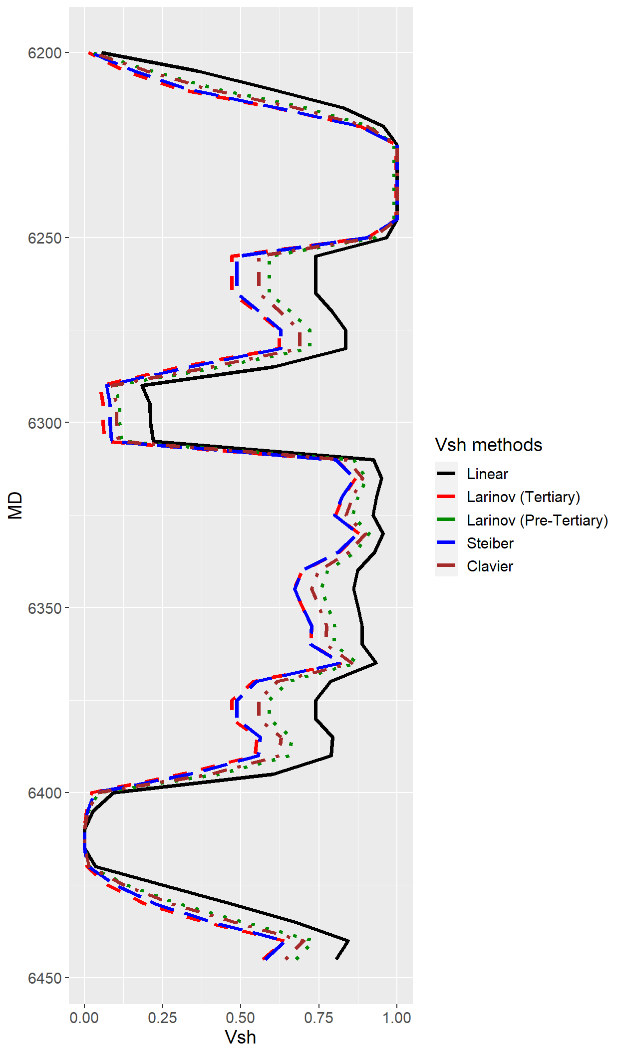
Now, we can calculate Gamma Ray Index and Shale content (\(V_{sh}\)) using the equations above.

Vsh <- log_data %>%
        mutate(IGR = (GR-58.12)/(111.86-58.12),
               IGR = ifelse(IGR>1, 1, IGR),
               IGR = ifelse(IGR<0, 0, IGR),
               Vsh_Linear = IGR,
               Vsh_LarionovUn = 0.083*(2^(3.7*IGR)-1),
               Vsh_LarionovC = 0.33*(2^(2*IGR)-1),
               Vsh_Stieber = (0.5*IGR)/(1.5-IGR),
               Vsh_Clavier = 1.7-(3.38-(IGR+0.7)^2)^0.5)  %>%
        select(MD, IGR, Vsh_Linear, Vsh_LarionovUn, Vsh_LarionovC, Vsh_Stieber, Vsh_Clavier)

datatable(Vsh)

plot_Vsh <- ggplot(Vsh) + geom_line(aes(MD,Vsh_Linear, colour = "Linear"), size = 1.25) +
            geom_line(aes(MD,Vsh_LarionovUn, colour = "Larinov (Tertiary)"), linetype = "dashed", size = 1.25) +
            geom_line(aes(MD,Vsh_LarionovC, colour="Larinov (Pre-Tertiary)"), linetype = "dotted", size = 1.25) +
            geom_line(aes(MD,Vsh_Stieber, colour = "Steiber"), linetype = "longdash", size = 1.25) +
            geom_line(aes(MD,Vsh_Clavier, colour = "Clavier"), linetype = "dotdash", size = 1.25) +
            coord_flip() + ylab("Vsh") +
            scale_x_continuous(trans = "reverse") +
            theme(text = element_text(size=14), legend.position="right") +
            scale_color_manual(name = "Vsh methods", breaks = c("Linear", "Larinov (Tertiary)",
                                                                  "Larinov (Pre-Tertiary)",
                                                                  "Steiber","Clavier"),
                                        values = c("black", "red" , "green4", "blue","brown"))

plot_Vsh

#ggplotly(plot_Vsh)

Files

References Sanni, M. (2019) Petroleum Engineering. Principles, Calculatios, and Workflows